Mixing efficiency

Mixing Efficiency

Aim

To understand the mixing phenomena of a Tee-joint by means of numerical simulations utilizing the Finite volume method and CFD technique. In the current study air at two different temperature is mixed using the Tee junction and the outlet temperature & enthalpy are studied. In addition we compare two popular turbulence models the k-ω SST model and the k-ɛ model, also understand grid independency. This problem has wide practical applications in the petrochemical industries, HVAC industry, pipeline sector, nuclear power plants.

Solving & Modelling approach

The fluid volume is extracted from the provided CAD model, wet volume obtained from the Spaceclaim is meshed i.e discretized which becomes the computational domain and for ease of identification while setting up the physics appropriate names are given to the boundary surfaces. The computational domain is applied with appropriate physical models in this case the RANS along with the turbulence model as well as energy equations. Then most importantly correct boundary conditions are applied (velocity inlet, pressure outlet, and no-slip wall). The equations get solved and we monitor its convergence using residuals.

Methodology:

1. Run base case simulation for two different turbulence models, to select a suitable turbulence model.
2. Perform grid independence study and choose a suitable grid size.
3. Perform the required simulation to understand the effect of momentum ratio & length of the tee in mixing.
4. Make inferences from the performed simulation and find areas of improvement if any.

Pre-processing

The first step is to import the given CAD model to Spaceclaim and extract the fluid (wet) volume from the provided CAD model as illustrated below.

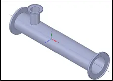
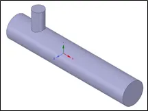
Fig: CAD preparation

There are two models the short tee of length 0.192m & long tee of length 0.2683m, with the inlet area of cold air & hot air being 0.0002 m² & 0.0009m² respectively for short tee as well as the long tee. We can use the measure feature Spaceclaim to find these dimensions. The next step would be to mesh the CAD model utilizing the ANSYS mesh module and also name the boundaries.

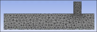
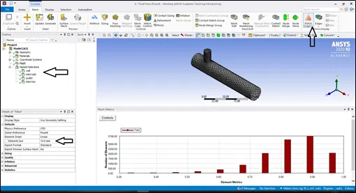
Fig: Meshing

Once the model has been meshed the next step would be setting up the physics of the problem using ANSYS FLUENT.

Setting up the physics

Once the mesh has been loaded to FLUENT, choose appropriate units of quantities from the units options, by default they will be SI units. The next step is to perform mesh check followed by clicking the energy option in “physics” tab since we need to measure temperature. In the “physics” tab open the viscous option and choose the required turbulence model.

The next step is to select the appropriate boundary conditions and assign values for the same, for example in the case of the short tee, with momentum ratio = 2 the inlet temperature and velocity of hot air is 36ºC & 3m/s, for cold air, it is 19ºC & 6m/s. In the outlet boundary condition, the gauge pressure by default is zero, and temperature by default is 26.78ºC. Once the boundary conditions are specified, one has to make report definitions so that we can obtain data of temperature, enthalpy so that we may be able to calculate the average outlet temperature and enthalpy at the end of the simulation. We then have to initialize the solution by clicking the hybrid option. Then specify the number of iterations that need to be run and hit on calculate. Check for convergence based on the residuals, once the solution has converged compute the average outlet temperature from the report definitions options under the solutions tab, and check with the analytically calculated outlet temperature. Then post-process the data and obtain the required plots.

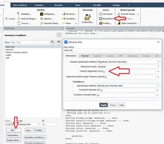
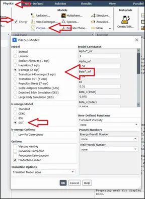
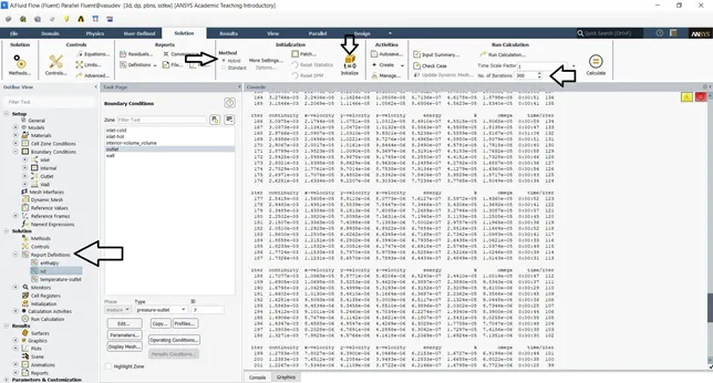
Fig: Setting up the physics

Solution

The base case of the short tee with momentum ratio = 2 was simulated with both realizable k-ɛ model & k-ω SST model, the k-ω SST model was chosen for all further simulations because the outlet temperature obtained from the k-ω SST model was found be closer to the analytically obtained solution with help of reference formulae. And also the k-ω SST models combines a little of both the k-ω & k-ɛ models and literature shows the k-ω SST model is used for problems involving parameters near the walls.

A grid independence study was performed by using three different element sizes namely 10mm, 7mm & 5mm.

	mesh study
Size	5mm	7mm	10mm
T-Outlet (ºC)	30.25657	30.23402	30.23101
%	0.074513	0.009962288	-

As the change in outlet temperature when the mesh size is varied falls well below 5%, the 10 mm grid size has been chosen for all further simulations.

CASE-1 SHORT TEE FOR 2 MOMENTUM RATIOS. 

The short tee, where hot inlet conditions are : Velocity = 3m/s & Temp = 36 ºC are run for two momentum ratios that two different cold air velocity inlet of 6m/s & 12 m/s, the temperature of cold air is 19 ºC.

Case-1	No of Iterations to Converge	Outlet-Temperature	cell count
m=2	216	30.231	12583
m=4	197	27.558	12583

The above table lists the no of iterations at which solutions converged and the outlet temperature at convergence. The figure given below shows the convergence plot for both.

 

Fig: Case1/m=2 convergence

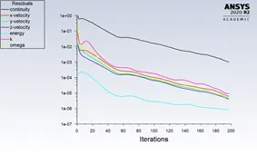
Fig: Case1/m=4 convergence

The first case where m=2 implies cold air inlet velocity is 6m/s, the outlet temperature obtained from the numerical method was found to be 30.23 ºC which close to the analytical value of 30.7 ºC. Temperature and velocity plots were made for both along and across the tee-pipe and they are given below.

The first three figures provide the velocity contour plots along  and across the short tee pipe, the inlet velocity of hot and cold air are 3 & 6 m/s respectively, while the outlet air achieves a velocity of 4m/s. In case of temperature, the hot & cold air temperature at the inlet was 36 ºC & 19 ºC, the average outlet temperature is 30.23 ºC

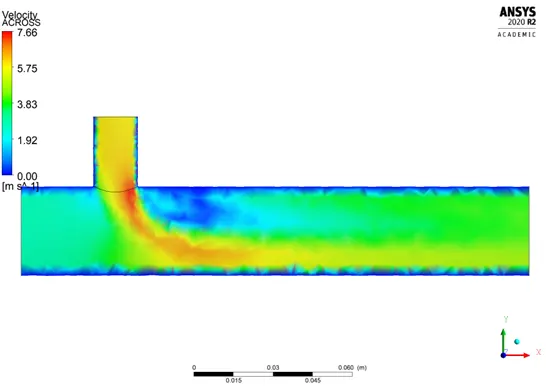
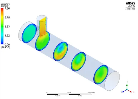
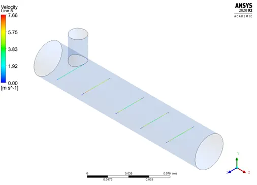
Fig: Velocity plots for various orientation for short tee/m=2.

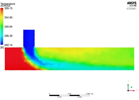
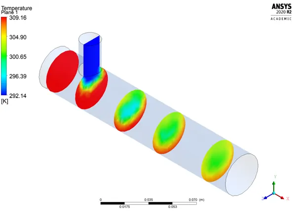
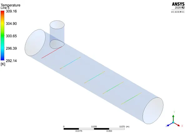
Fig: Temperature plots for various orientation for short tee/m=2.

When m=4; the velocity of cold air at the inlet becomes 12 m/s and the remaing settings and boundary conditions remain the same. The average outlet temperature was obtained to be 27.558 ºC which is only 1.5% less than the analytical solution of 28 ºC. The flow behaviour has been plotted and are present below

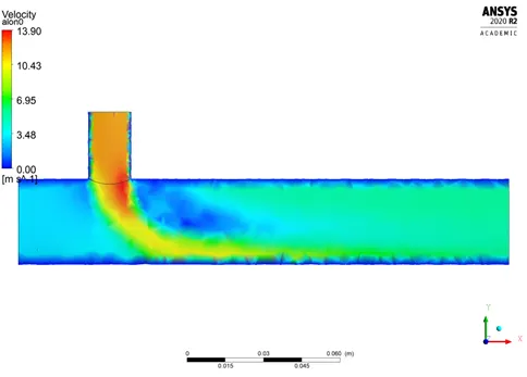
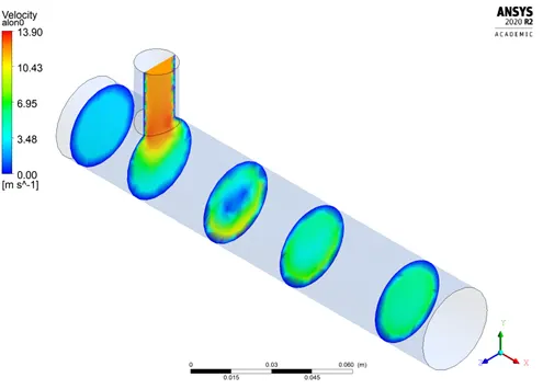
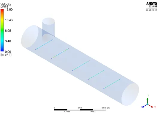
Fig: Velocity plots for various orientation for short tee/m=4.

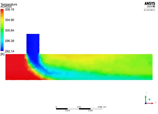
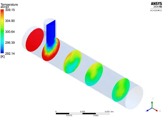
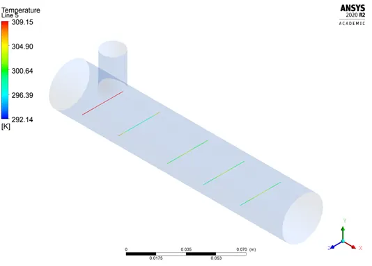
Fig: Temperature plots for various orientation for short tee/m=4.

It can be found that larger momentum ratios (larger velocities) are more suitable for this application because of the better-cooled air at the outlet of 27.558 ºC.

CASE-2 LONG TEE FOR 2 MOMENTUM RATIOS.

 In this case we will be simulating the same inlet conditions of hot air & cold air

Temperature & velocity of hot air: 36 ºC & 3m/s

Temperature & velocity of cold air: 19 ºC & 6 (m=2), 12 (m=4) m/s for longer tee pipe of length 0.2683m.The table given below shows the no of iterations it took for convergence & the average outlet temperature.

Case-2	No of Iterations to Converge	Outlet-Temperature	cell count
m=2	175	30.31735	15384
m=4	129	27.486173	15384

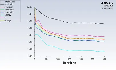
Fig convergence plot for long tee/m=2

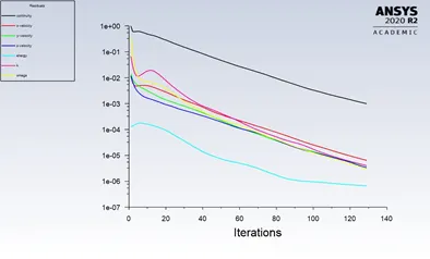
Fig convergence plot for long tee/m=4.

The following figures present the temperature & velocity contour plots obtained for m=2. The average outlet temperature in this case is found to be 30.31 ºC which lightly larger than temperature obtained in shorter tee. The velocity at the outlet can also be found to be slightly lower than short tee velocity.

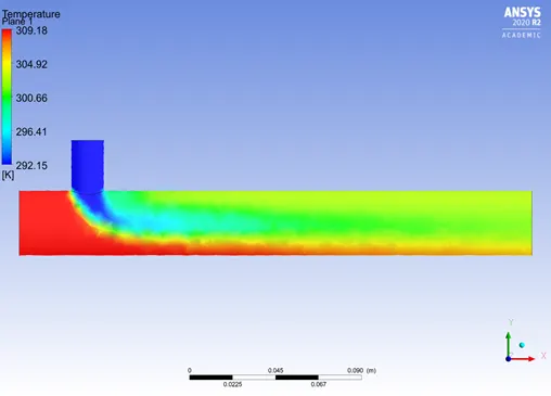
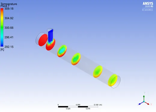
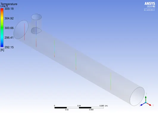
Fig: temperature plots for long tee & m=2.

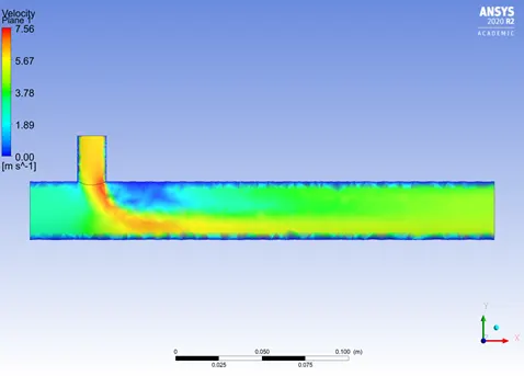
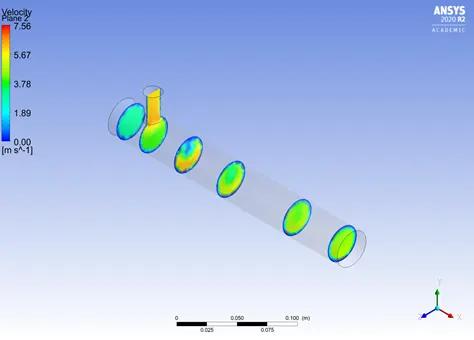
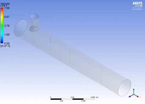
Fig: velocity for long tee & m=2.

In the second part, we will be simulating the flow when the cold air inlet velocity is 12 m/s i.e. momentum ratio = 4, while the remaining parameters remain the same. The temperature & velocity contour plots for case-2 (long tee) & m=4 is shown below.

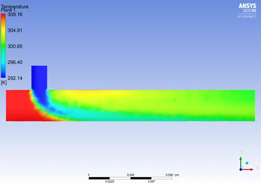
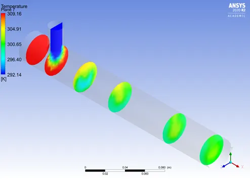
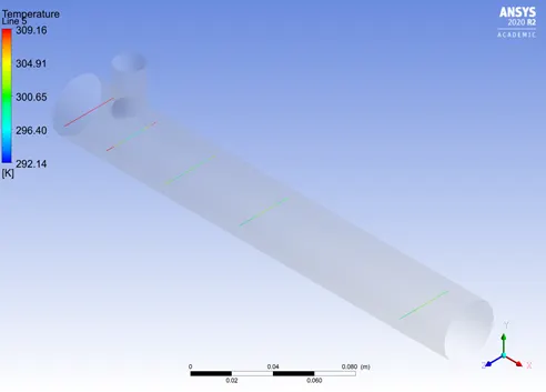
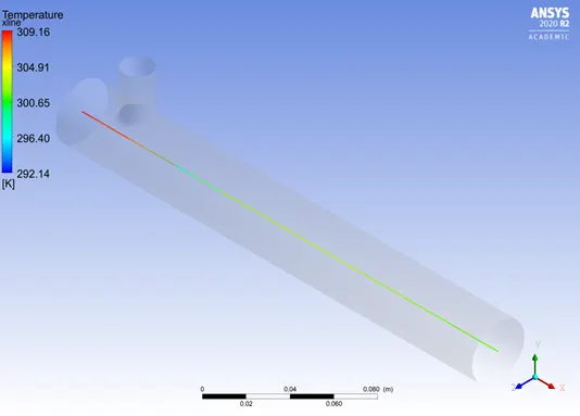
Fig: Temperature plots for long tee with m=4

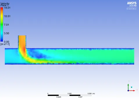
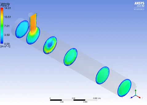
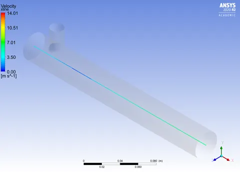
Fig: velocity plots for the long tee with m=4.

The longer length can be found to have very little or no significant impact on the outlet temperature.

Results & Discussions

The following table summarises both cases being studied in terms of the number of iterations, average outlet temperature & cell count.

Case-1	No of Iterations to Converge	Outlet-Temperature	cell count	analytical Temperature	% change
m=2	216	30.231	12583	30.76923077	1.74925
m=4	197	27.558	12583	28	1.578571
Case-2	No of Iterations to Converge	Outlet-Temperature	cell count	analytical Temperature	% change
m=2	170	30.31735	15384	30.76923077	1.468612
m=4	129	27.486173	15384	28	1.835096

The following table show the analytical calculation performed in excel sheet with help of reference formulae for m=2.

Analytical Temperature Calculation
Area.hot	0.0009	velocity.hot	3	mass flow rate.hot	0.0033075	Temp.hot	36
Area.cold	0.0002	velocity.cold	6	mass flow rate.cold	0.00147	Temp.cold	19
		momentum ratio	2			Temp.mixture	30.76923077

Conclusion:

• A larger Momentum ratio is more suited in case of cooling application as it significantly lowers the outlet temperature.
• In terms of length, the outlet temperature is slightly effected.
• For further study, the effect of pipe material can be studied on the outlet temperature.