Objective :- To simulate the multiphase fluid transient interaction to study the Rayleigh Taylor Instability and effects of mesh size on results.

Introduction :-

Rayleigh Taylor instability- is an instability of an interface between two fluids of different densities which occurs when the lighter fluid is pushing the heavier fluid. Water suspended atop oil is an everyday example of Rayleigh–Taylor instability,heavier fluid is displaced downward with an equal volume of lighter fluid displaced upwards, the potential energy of the configuration is lower than the initial state. Thus the disturbance will grow and lead to a further release of Potential energy, as the more dense material moves down under the (effective) gravitational field, and the less dense material is further displaced upwards. This was the set-up as studied by Lord Rayleigh.

G. I. Taylor found an important insight that Rayleigh's interfacial instability also occurs for accelerations other than gravity, this situation is equivalent to the situation when the fluids are accelerated, with the less dense fluid accelerating into the more dense fluid.

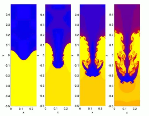
Practical CFD models that have been based on the mathematical analysis of Rayleigh Taylor waves?

Kelvin-Helmholtz instability - typically occurs when there is velocity shear in a single continous fluid or additionally where there is a velocity difference across the interface between two fluids.This instability can be observed & used in

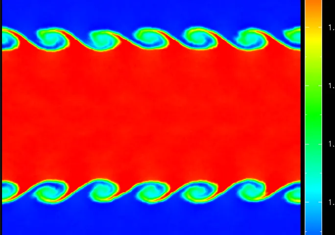
• Natural phenomenon of certain cloud patterns.
• An improved spray atomization model is developed for use in both diesel and gasoline spray computations,KH instability model was used to predict the primary breakup of the intact liquid core of a diesel jet,secondary breakup of the individual drops was modeled by KH-RT hybrid model and was also found to predict the spray shape, penetration, and local hollow-cone sprays as well as previous gasoline spray models & to improve the temperature dependence of the liquid fuel penetration of the diesel sprays significantly.
• KHI model dynamics and their implications are used for airglow observations,interpretations and the increasing ability of airglow imaging, radars, and lidars.
• To analyse the solar corona is its heating mechanism. Scientists have suggested that MHD waves propagating on flowing magnetic flux tubes can become unstable as the flow speed exceeds some critical value, and the developing KH instability might trigger turbulence, which causes heating.

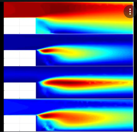
KL turbulence model -

• Is a two-equation turbulence model developed to describe the self-similar growth of the Rayleigh-Taylor (RT) and Richtmyer-Meshkov (RM) instabilities.
• The dominant eddies in the mixing zone with evolutionary equations for their turbulent eddy scale length(L) and kinetic energy(k) per unit mass `K = V^2/2`
• The equations are based on the successful buoyancy-drag models for RT and RM flows, but constructed only with local parameters so that it can be applied to multidimensional flows with multiple shells of materials.

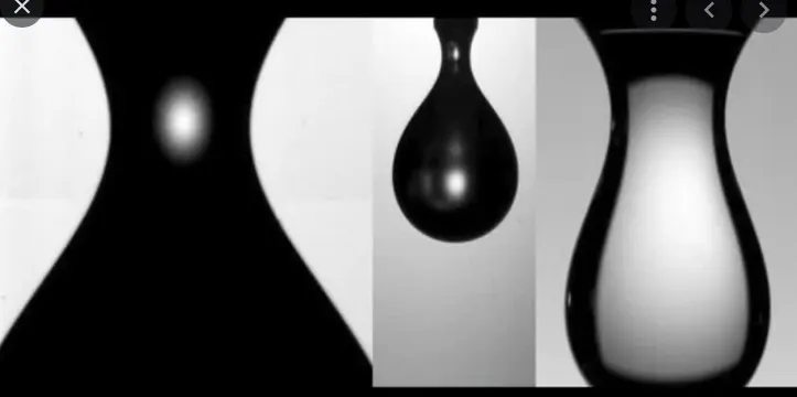
Plateau-Rayleigh instabilty - explains why and how a falling stream of fluid breaks up into smaller packets with the same volume but less surface area. It is related to the RT instability and is part of a greater branch of fluid dynamics concerned with fluid thread beakup.The driving force of the Plateau–Rayleigh instability is that liquids, by virtue of their syrface tensions, tend to minimize their surface area.

• This fluid instability is exploited in the design of a particular type of Ink jet technology. whereby a jet of liquid is perturbed into a steady stream of droplets.

Geometry :-

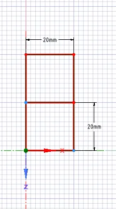
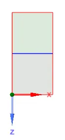
For a 2D simulation, two square surfaces component of size 20x20mm is created with common intersection.

Shared topolgy - share prep is done for both bodies & coincident toplogy is shared at adjoing edge to obtain a even mesh on both bodies & at intersection.We can confirm by checking the icon change & in properties share topology will be enabled automatically.

Case 1 :

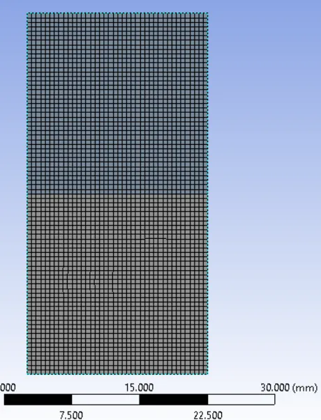
As base mesh will start analysis with 0.5mm element size.

• Meshing

• Fluent setup setting-

(why a steady-state approach might not be suitable for these types of simulation ?)

As we are intersted in capturing interface collapsing over the time before attaining steady sate mixture.Transient state simulation is opted for solving & to observe the intersting Rayleigh Taylor instability phenomenon b/w two different phases of fluid.

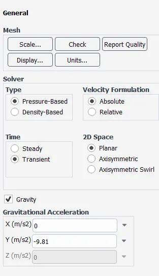
Gravity is tuned 'On' and value provided in negative direction (gravity acting downwards Y-)

Viscous Model -

Laminar (As velocity is low/simple)

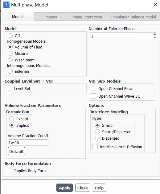
Multiphase model - Multiphase flows can be numerically calculated using either Euler- Lagrange approach or Euler-Euler approach. VOF (Volume of Fluid method)is a type of Euler-Euler approach, it is basically a surface tracking technique. Usually used if there are more than two immersible fluids, where interface position is of importance.

Implicit method formulation is done.

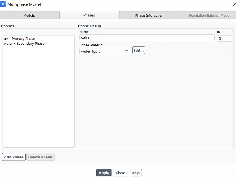
Materials - Two immiscible fluids

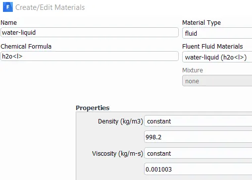
1. Water (denser)
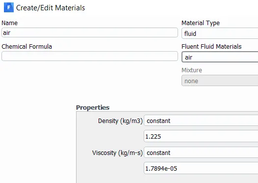
2. air (lighter)

Material property -

Solution Intialization-

Standard Intialization is done,as there is no proper inflow or outflow.

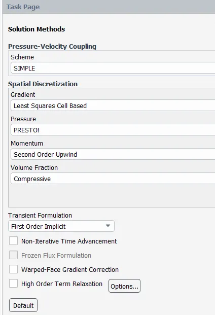
Changing Discretization Scheme for Pressure to PRESTO!

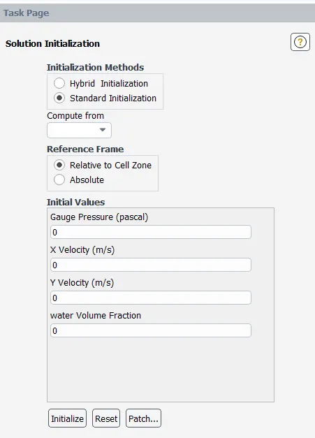
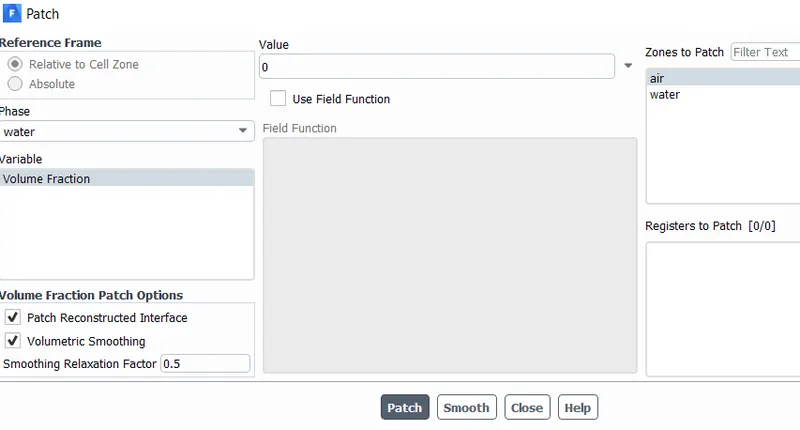
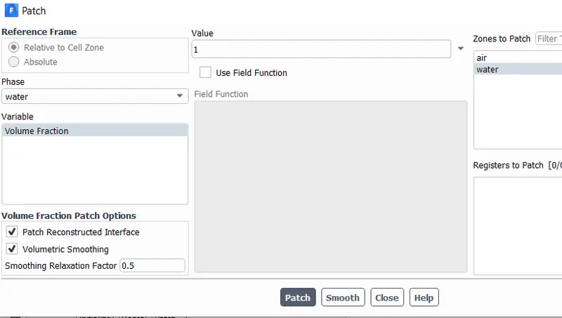
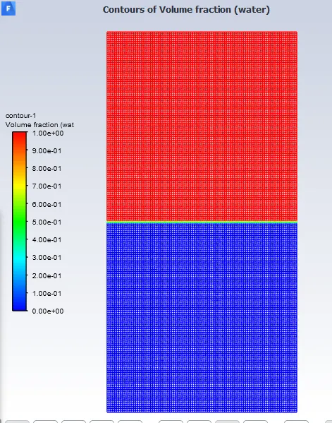
Phases are patched - The two phases are represented basically reperesented by `alpha` with value 1 or 0, to ensure denser material(water) in top & air below. To

water value =1 ; air value = 0

To confirm correct intialization a VOF contour of water phase is plotted

Run Calculation -

time step -0.005

no. of time steps = 300

max. iterations/time step =20

Results -

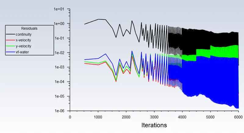
Scaled residual plot:

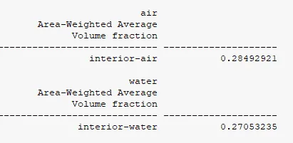
VOF values -

VOF contours of water & air-

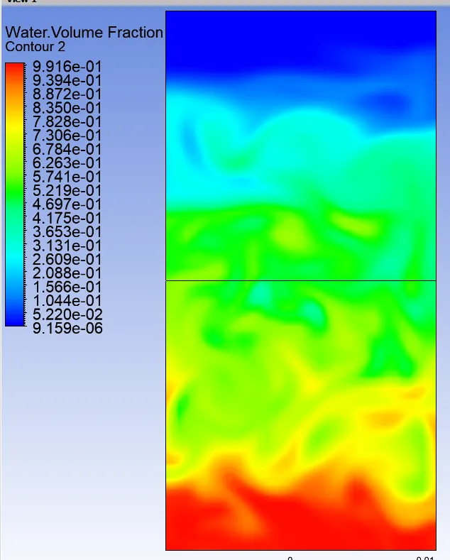
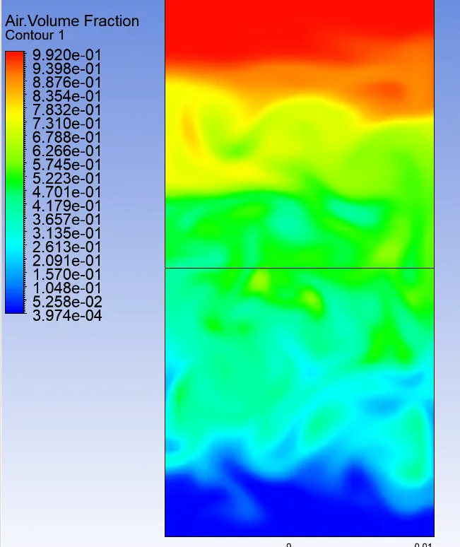
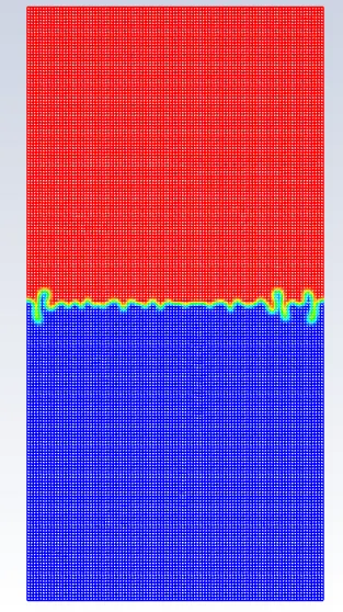
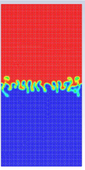
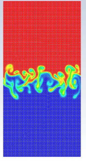
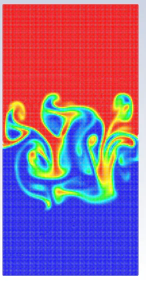
Rayleigh Taylor Instability development stages -

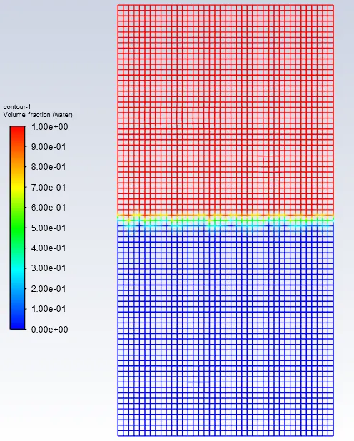
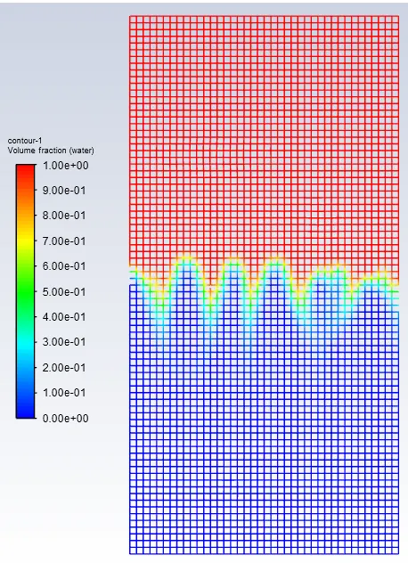
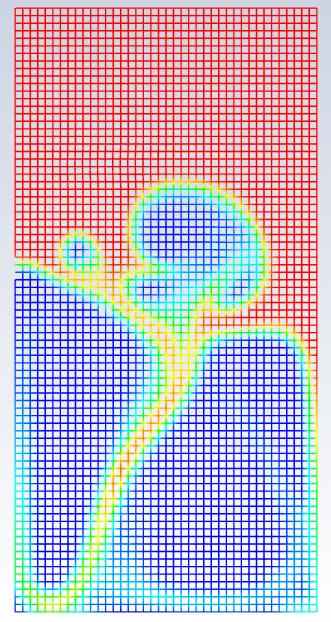
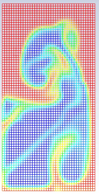
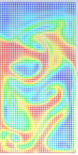
Animation video link on Youtube -https://youtu.be/Yu2rAmktkio

Case 2a : Refined mesh

Element size = 0.2mm

No. of elements = 20000

Run Calculation -

time step -0.005

no. of time steps = 200

max. iterations/time step =20

Results -

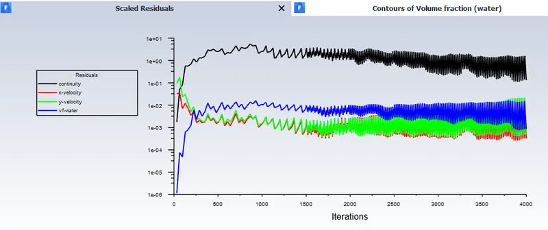
Scaled residual plot:

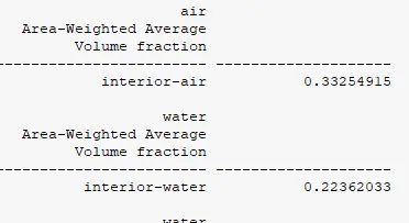
VOF values -

VOF contours of water & air -

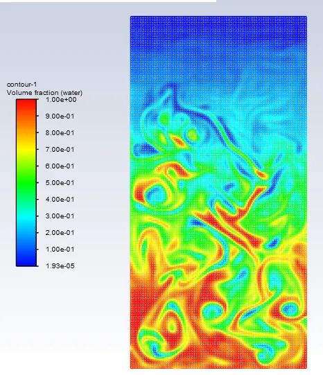
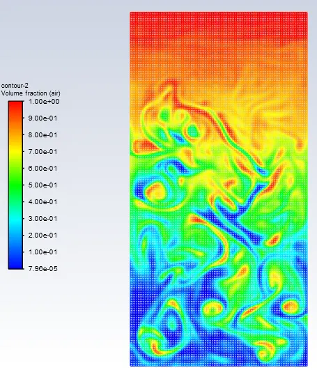
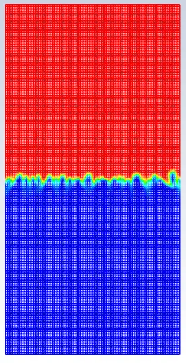
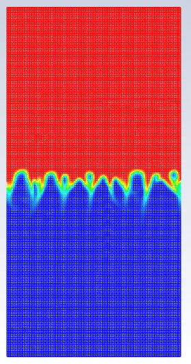
Rayleigh Taylor Instability development stages -

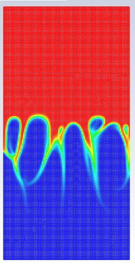
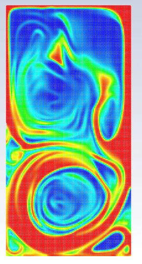
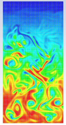
Animation video link on Youtube - https://youtu.be/KwodRL4i4Fc

Case 2b - custom fluid material (Refined mesh)

Instead of air & user-defined fluid having below attached properties , used to observe the change in results.

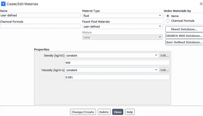
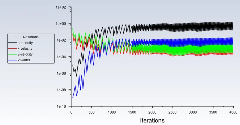
Results -

Scaled residual plot:

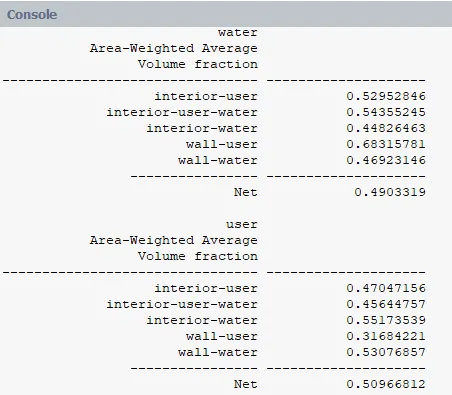
VOF values -

Animation video link on Youtube - https://youtu.be/B3pFL_okXIo

VOF contours of water & custom fluid -

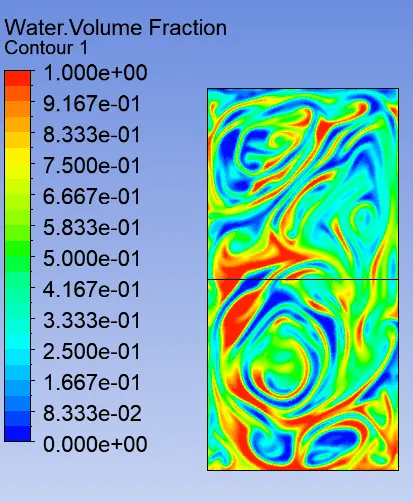
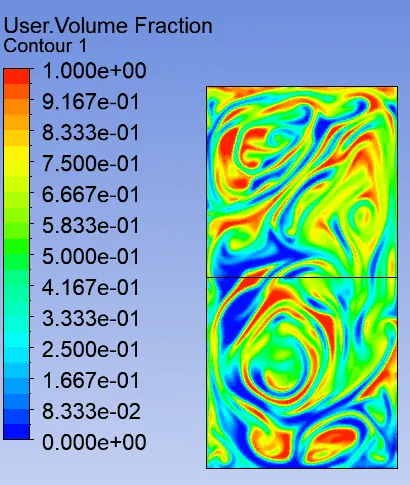
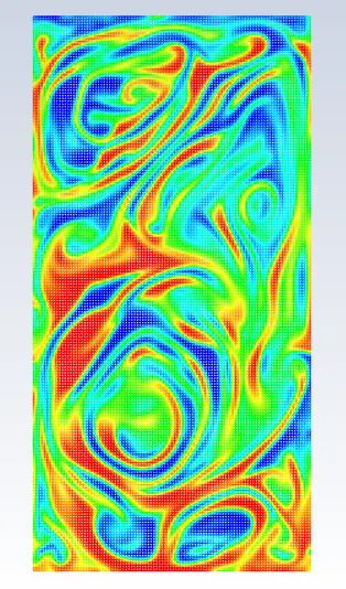
Rayleigh Taylor Instability development stages -

Atwood Number :

• Is a dimensionless number in fluid dynamics used in the study of hydrodynamic instabilities in density stratified flows. It is a dimensionless density ratio defined as

`A = (rho1 - rho2)/(rho1 + rho2)`

Where, `rho1`= density of heavier fluid

`rho2`= density of lighter fluid

• Atwood number is an important parameter in the study of RT instability, the penetration distance of heavy fluid bubbles into the light fluid is a function of acceleration time scale

Calulation -

For case 2a :

Air density = `rho1`=1.225 kg/m^3

water density = `rho2`= 1000 kg/m^3

`A = (1.225-1000)/(1.225+1000) = 0.997`

For case 2b :

custom fluid density = 400 kg/m^3

`A = (1.225-400)/(1.225+400) =0.428`

• Atwood no. ranges from 0 to 1, which significantly discribes the trasient fluid interaction.
• For case2a A =0.997 higher density difference causing heavier fluid to spike down fast & turbulent instablity arises with effective mixing.
• For case2b A=0.428 lighter density difference causing a laminar instabilty due to viscosity difference.