Week 5 - Rayleigh Taylor Instability

AIM:

To perform the Rayleigh Taylor Instability for the geometry with two different mesh sizes and have to observe the differences between instability. Have to understand the concept of Atwood number. Have to create the new material using the data provided and run the simulation using the water and new material.

THEORY:

Rayleigh Taylor Instability:

Rayleigh Taylor instability is an instability of an interface between two fluids where different densities are there. The stability occurs when the high-dense fluid is placed over the low-dense fluid under gravitational force. The perturbation will grow further to the release of potential energy, as the denser material moves down under the effective gravitational field and the less denser material is displaced upwards. This setup was done by Lord Rayleigh.

The important insight by GI Taylor was the realization that this situation is equivalent to the situation when the fluids are accelerated.

Stages of RT Instability:

RT Stability follows four main stages.

First Stage - Perturbation amplitudes are small when compared to their wavelength, the equation of motion can be linearized, resulting in exponential instability growth. In this stage, sinusoidal initial perturbations will remain in sinusoidal shape.

Second Stage - In this stage, non-linear effects begin to appear, and we can observe the mushroom-shaped spikes(heavy fluid growing into the lighter fluid) and bubbles(light fluid growing into heavy fluid). The growth of mushroom structure continues in the second stage and can be modeled by the buoyancy drag model, resulting in a growth rate that is approximately constant in time.

Third Stage - Bubble merging takes place in this stage where the non-linear mode of coupling acts to combine smaller spikes and bubbles to produce larger ones. Then the bubbles and spikes of smaller wavelengths that have become saturated are enveloped by larger ones that have not yet saturated. Baroclinic torque occurs and creates vorticity.

Fourth Stage - THis is the mixing region that developed self-similar and turbulent, provided that reynolds number is sufficiently large.

Ritchmyer-Meshkov instability:

The Richtmyer-Meshkov instability arises when a shock wave interacts with an interface separating two different fluids. It combines compressible phenomena, such as shock interaction and refraction, with hydrodynamic instability, including nonlinear growth and subsequent transition to turbulence, across a wide range of Mach numbers.

Plateau–Rayleigh instability:

The Plateau–Rayleigh instability, often just called the Rayleigh instability, explains why and how a falling stream of fluid breaks up into smaller packets with the same volume but less surface area. This fluid instability is exploited in the design of a particular type of ink jet technology whereby a jet of liquid is perturbed into a steady stream of droplets.

Kelvin–Helmholtz instability:

can occur when there is velocity shear in a single continuos fluid, or where there is a velocity difference across the interface between two fluids. An example is a wind blowing over water: The instability manifests in waves on the water surface. More generally, clouds, the ocean, Saturn's bands, and the sun's corona show this instability.

Practical CFD models:

SPH method(Smoother particle hydrodynaics)

Smoothed-particle hydrodynamics (SPH) is a computational method used for simulating the mechanics of continuum media, such as solid mechanics and fluid flows.Smoothed-particle hydrodynamics is being increasingly used to model fluid motion as well. This is due to several benefits over traditional grid-based techniques. First, SPH guarantees conservation of mass without extra computation since the particles themselves represent mass. Second, SPH computes pressure from weighted contributions of neighboring particles rather than by solving linear systems of equations. Finally, unlike grid-based techniques, which must track fluid boundaries, SPH creates a free surface for two-phase interacting fluids directly since the particles represent the denser fluid and empty space represents the lighter fluid.

INTRODUCTION:

For this problem we are going to create three cases

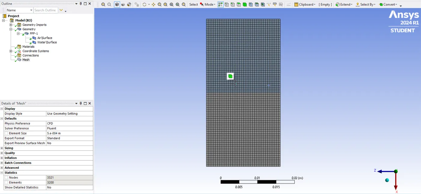
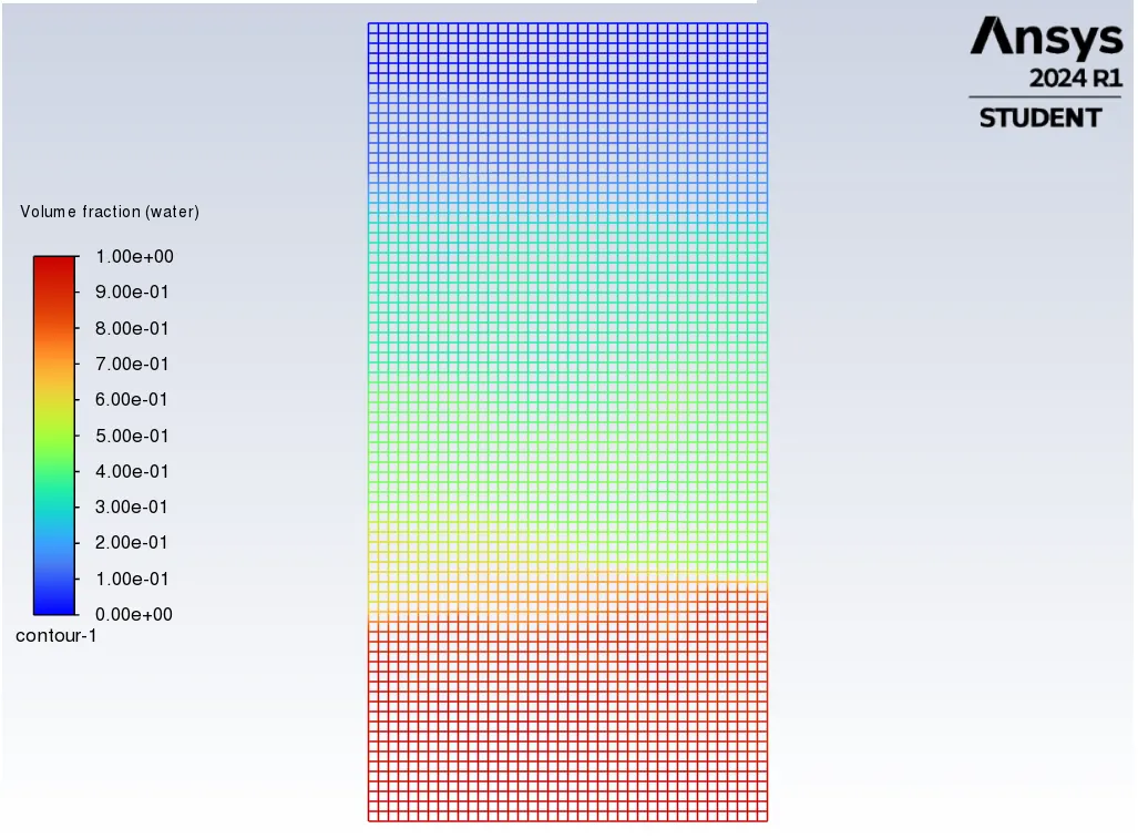
CASE I: Rough meshing with the size of 0.5mm; Use of Air and Water Medium

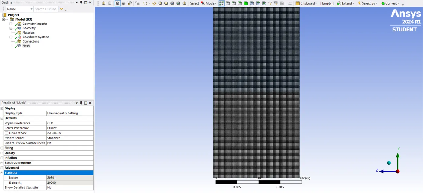
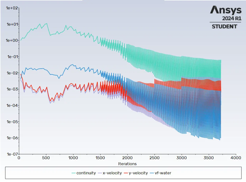
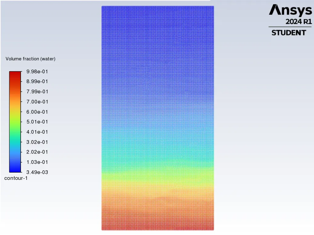
CASE II: Meshing refinement is done with the size of 0.2mm; Use of Air and Water Medium

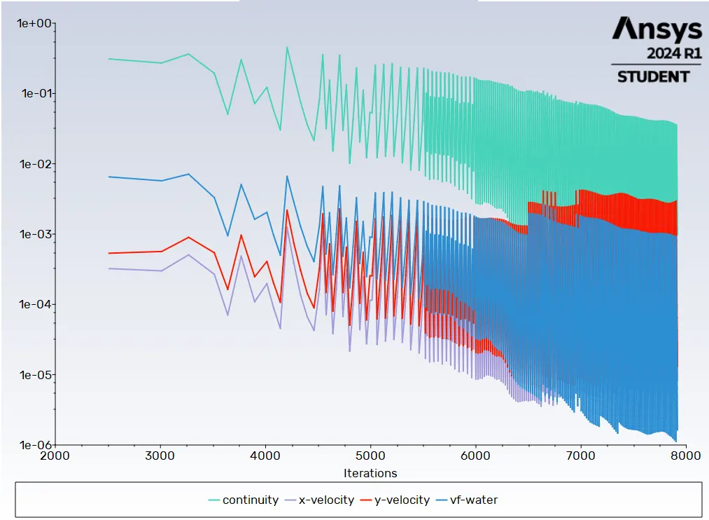
CASE III: With the mesh size of 0.2mm; Use of Water and Used Defined Material as a medium

PROCEDURE:

GEOMETRY SETUP:

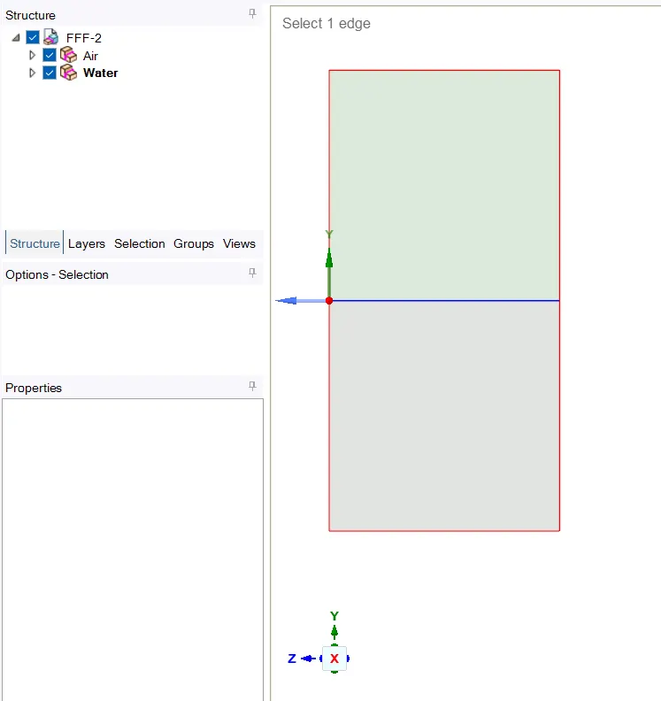
Create the geometry in the space claim, for two different components as air and water. Provide the share preparation for sharing the topology between the two surfaces.

MESHING:

Now we can mesh the geometry. As we already discussed we are going to do the meshing by three different cases to understand the concept of Rayleigh Taylor Instability.

CASE I:

Meshing Size - 0.5mm

CASE II & CASE III:

Meshing Size - 0.2mm

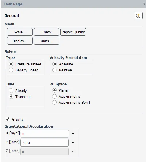
METHOD SELECTION:

Turbulence Model : Laminar

Solver : Pressure Based Solver

Time : Transient

Method : SIMPLE (Semi-Implicit Method for Pressure Linked Equation)

Working Fluid : Air (with standard values) & Water (with standard values)

Then the materials are choosed respectively from the fluent database.

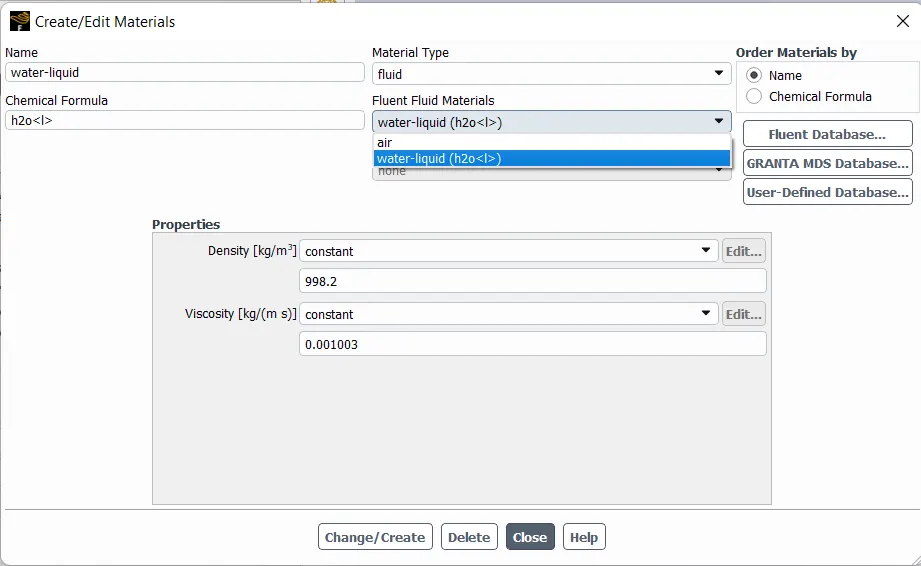
Then the choosen materials are assigned to the respective surfaces.

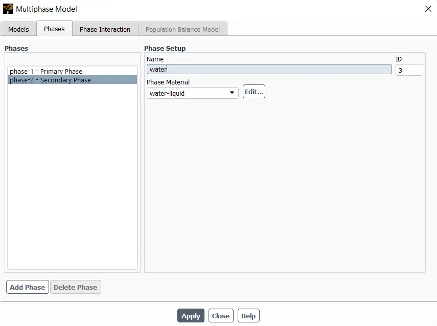
Then the initialization is done. After the initialization is done, we have to do the patching to align the surfaces to the material values.

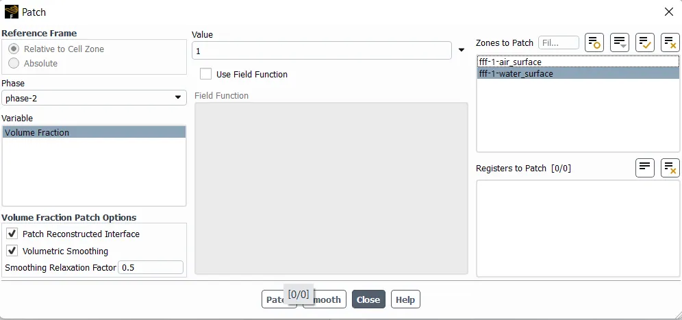
PLOT:

CASE I:

Residuals:

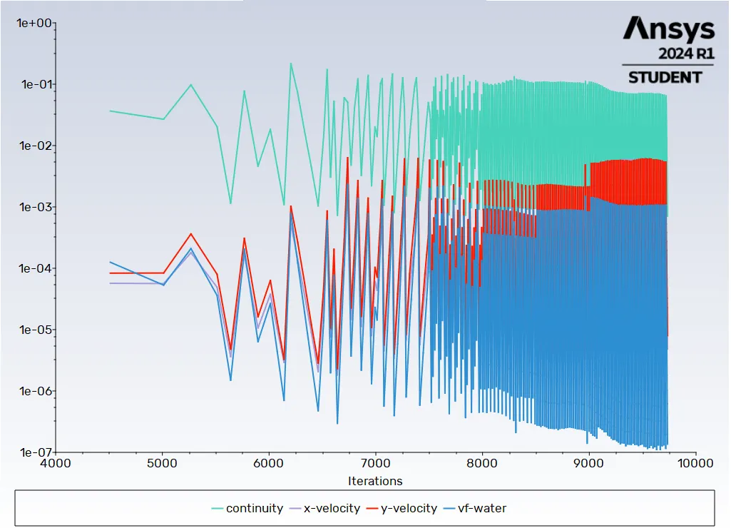
Contour after mixing:

CASE II:

Residuals:

Contours after mixing:

OBSERVATION FROM CASE I and CASE II:

With the coarse mesh it is observe that earlier bubble separation occurs which dominates the strike formed at the initial stage. And also the solution goes to non linear at the initial stage due to the coarse meshing. Whereas in the refined mesh, the equation of motion is linearized in the initial stage which form the sinusoidal initial perturbations resulting in the exponential instability growth. And then due to the high density difference the bubble separation occurs and the solution merges equally.

Thus the refined mesh captures the initial stages of sinusoidal perturbations and the instability growth is exponential.

CASE III:

Turbulence Model : Laminar

Solver : Pressure Based Solver

Time : Transient

Method : SIMPLE (Semi-Implicit Method for Pressure Linked Equation)

Working Fluid : Water (with standard values) & Used Defined Material ( Density - 400 kg/m3 ; Viscosity - 0.001 kg/m.s)

Residuals:

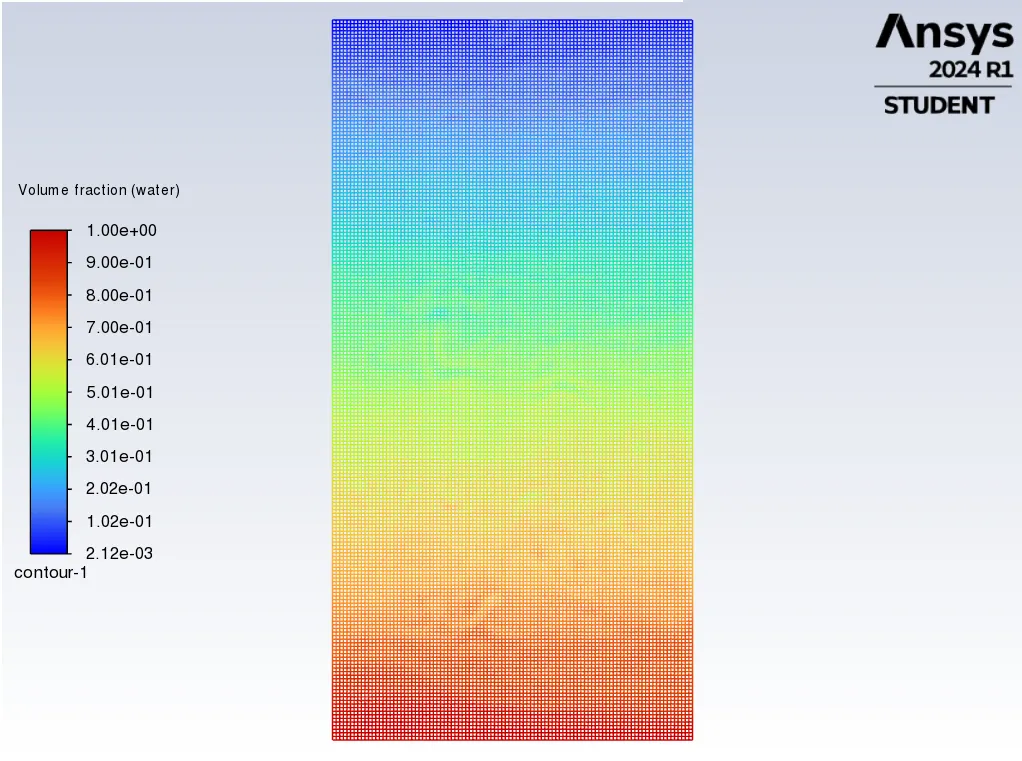
Contour after Mixing:

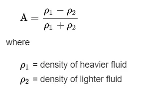
ATWOOD NUMBER:

Atwood number is a dimensionless number in fluid dynamics used in the study of hydrodynamic instabilities in a density stratified flows. It characterizes between the density differences between the two fluids.

For A which is closer to 0 the RT Instability flow takes the form of symmetric fingers of fluid; For A which is closer to 1 the much lighter fluid below the heavier fluid takes the large bubble like plumes.

Atwood number for above cases:

CASE-II:

A=998.2−1.225998.2+1.225=996.975999.425=0.9975�=998.2-1.225998.2+1.225=996.975999.425=0.9975

CASE-III:

A=998.2−400998.2+400=598.21398.2=0.4278

As stated by the law, by looking at the CASE II it is clearly seen that the less dense fluid of air takes the large bubble like plumes and flow over top. For the case of small Atwood number like CASE III, the density difference between the two sides of the interface is small, and the density distribution of upper and lowe layers is nearly symmetrical. The initial density stratification plays a dominant role, and the expansion-compression effect (Surface tension and gravity effect) has little influence. With the increase in the Atwood number, the stabilization effect of the initial density stratification decreases, and the instability caused by the expansion-compression effect becomes more significant.

CONCLUSION:

Thus the Rayleigh Taylor Instability is performed using the different meshing size and the differences of the results are observed. Then material is changed and the variation of Atwood number is achieved. With respect to the atwood number we clearly observed the variation of results.

LEARNING OUTCOMES:

• Phenomenon of Rayleigh Taylor Instability is learned
• Atwood number significance
• Volume of Fluid in Ansys Fluent