Week 5 - Rayleigh Taylor Instability

What are some practical CFD models that have been based on the mathematical analysis of Rayleigh Taylor waves? In your own words, explain how these mathematical models have been adapted for CFD calculations.

Rayleigh-Taylor instability (RTI) is the interpenetration of materials that occurs whenever a light fluid pushes on a heavy fluid. It is a dynamic process whereby the two fluids seek to reduce their combined potential energy. The ensuing turbulence and mixing has far-reaching consequences in many natural and man-made flows, ranging from supernovae to inertial confinement fusion (ICF) capsules.

Some practical CFD models that have been based on the mathematical analysis of Rayleigh Taylor waves are-

• Kelvin-Helmholtz instability - This instability typically occurs when there is velocity shear in a single continuous fluid, or additionally where there is a velocity difference across the interface between two fluids. A common example is seen when wind blows across a water surface; the instability constant is able to manifest itself through waves on water surface. The theory predicts the onset of instability and transition to turbulent flow in fluids of different densities moving at various speeds. 
• Richtmyer-Meshkov instability - This instability can be considered the impulsive-acceleration limit of the Rayleigh Taylor instability. This occurs when two fluids of different density are impulsively accelerated. Normally this is by the passage of a shock wave. The development of the instability begins with small amplitude perturbations which initially grow linearly with time. This is followed by a nonlinear regime with bubbles appearing in the case of a light fluid penetrating a heavy fluid, and with spikes appearing in the case of a heavy fluid penetrating a light fluid. A chaotic regime eventually is reached and the two fluids mix. 
• Plateau-Rayleigh instability - This instability, often just called the Rayleigh instability, explains why and how a falling stream of fluid breaks up into smaller packets with the same volume but less surface area. The driving force of the Plateau–Rayleigh instability is that liquids, by virtue of their surface tension, tend to minimize their surface area. This fluid instability is exploited in the design of a particular type of ink jet technology whereby a jet of liquid is perturbed into a steady stream of droplets.

Define the Atwood Number. Find out the Atwood number for both the cases and explain how the variation in Atwood number in the above two cases affects the behavior of the instability. 

The Atwood number (A) is a dimensionless number in fluid dynamics used in the study of hydrodynamic instabilities in density stratified flows. It is a dimensionless density ratio defined as:

A = (ρ₁-ρ₂)/(ρ₁+ρ₂)

Where, ρ₁ = density of Heavier Fluid

            ρ₂ = density of lighter fluid

=================================================================  

AIM

To simulate Rayleigh Taylor instability using ANSYS Fluent

OBJECTIVES

• Perform the Rayleigh Taylor instability simulation for 2 different mesh sizes with the base mesh being 0.5 mm. Compare the results by showing the animations( Attach them from your google drive). Observe the differences in the animation and explain the effect of mesh size on simulation. Also, explain why a steady-state approach might not be suitable for these types of simulation.[ Choose Air and Water for this simulation]
• Run one more simulation with water and user-defined material(density = 400 kg/m³, viscosity = 0.001 kg/m-s) for refined mesh. 

PRE-PROCESSING

Geometry

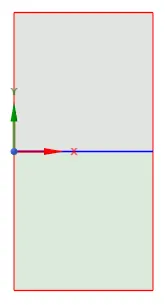
In SpaceClaim, a 2D geometry was created and a snapshot of the same is provided below. It shows two (20x20)mm² squares attached together vertically. The squares designate 2 immiscible fluids initaially separated by the interface. The topologies were shared to ensure a connected and conformed mesh.

 

Meshing

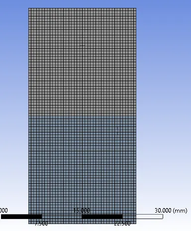
A base mesh was created with 3200 mesh elements where each mesh element had a size of 0.5 mm. 

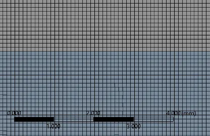
A refined mesh was created with 80k mesh elements where each mesh element had a size of 0.1 mm.

Solver

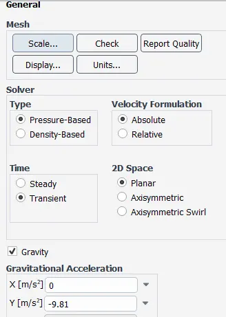
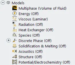
Presure based transient state solver was used for the simulations. Gravitational acceleration of 9.81 m/s² was applied in -y axis to imitate a vertically stacked setup. A laminar flow model was used alongwith a multiphase setup, which used the Volume of Fluids method to process the solution.

  

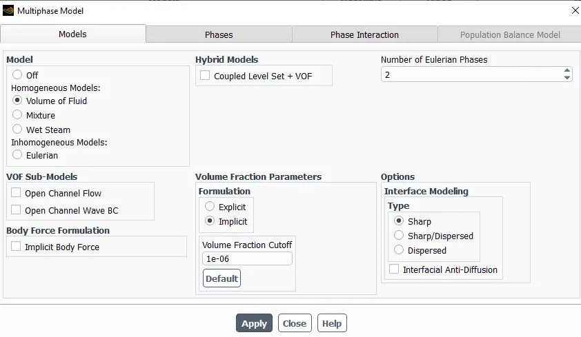
In the volume of fluids method setup, 2 eulerian phases were mentioned and implicit formulation was selected.

 

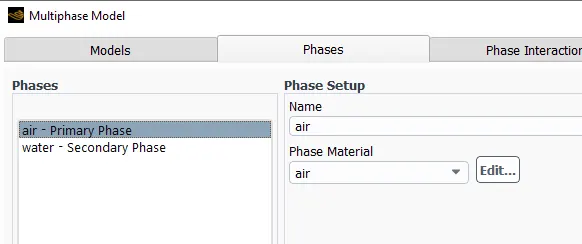
Initially, the phases were listed as air and water. While using the user defined material, primary phase was listed as user material and secondary phase was retained as water.

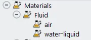
Below are snapshots of all 3 fluid materials used in the project.

  

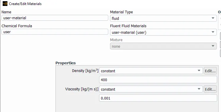
Properties of fluids

Fluid	Density (Kg/m3)	Viscosity (Kg/m-s)
Water	998.2	0.001003
Air	1.225	1.7894e-05
User defined material	400	.001

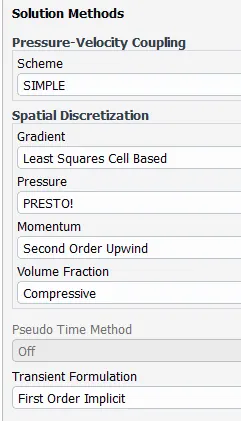
SIMPLE solution method was used and PRESTO! method was used to descretize the pressure equation.

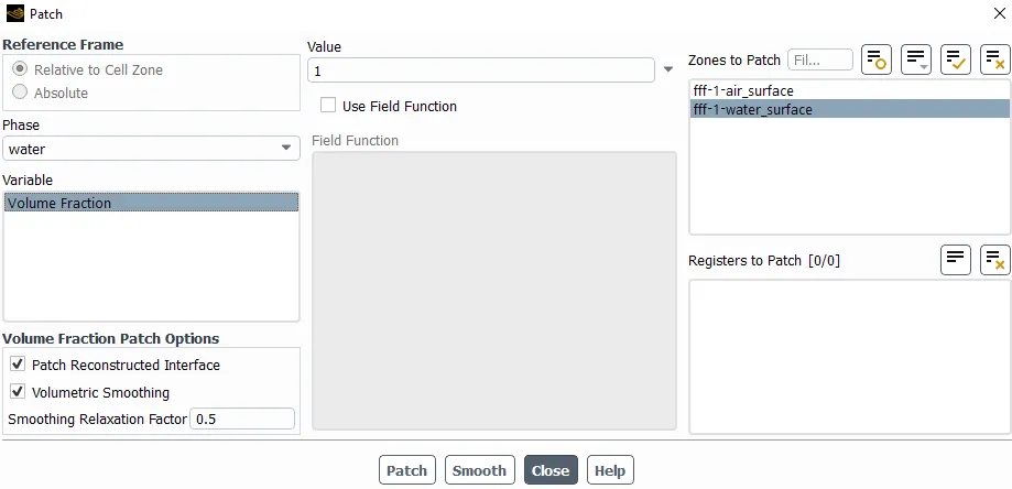
The setup was initialised using standard initialisation and the 2 fluid volumes were patched considering Volume Fraction variable. Water -1 , air - 0.

Additionally, Volume Fraction (Water) contour was created and the same was used for creating an animation of the solution.

Finally, the setup was run to calculate the solution.

Solution

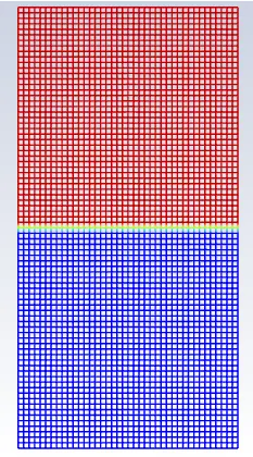
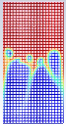
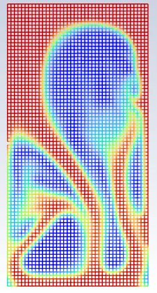
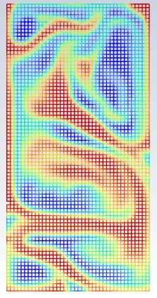
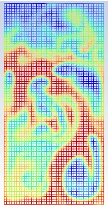
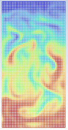
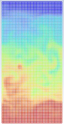
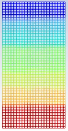
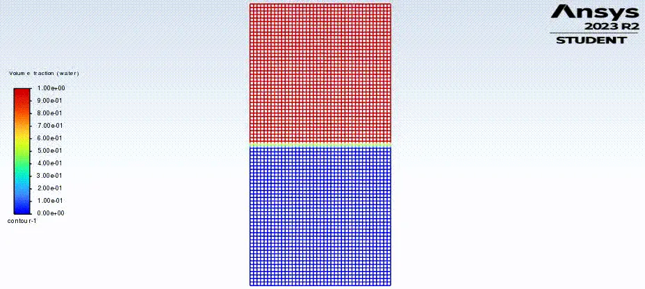
BASE MESH (3200 mesh elements) using water and air was run for 1500 timesteps with each timestep measuring 0.005 seconds. This generated an animation of the RTI phenomenon of 7.5 seconds. The same has been provided as a .gif file below.

Scaled residuals

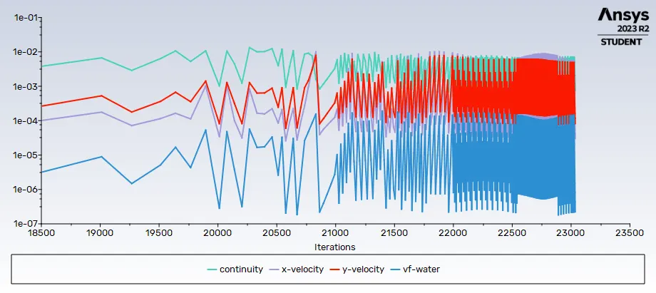
Different stages of the RTI phenomenon between water and air

Solution animation

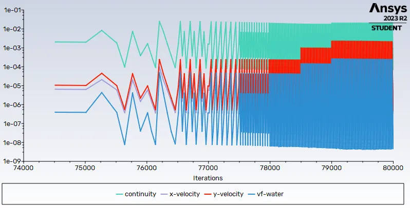
FINE MESH (80k elements) using water and air was run for 4000 timesteps with each timestep measuring 0.001 seconds. This generated an animation of the RTI phenomenon of 4 seconds. The same has been provided as a .gif file below.

Scaled residuals of 80k iterations

 

 Solution animation

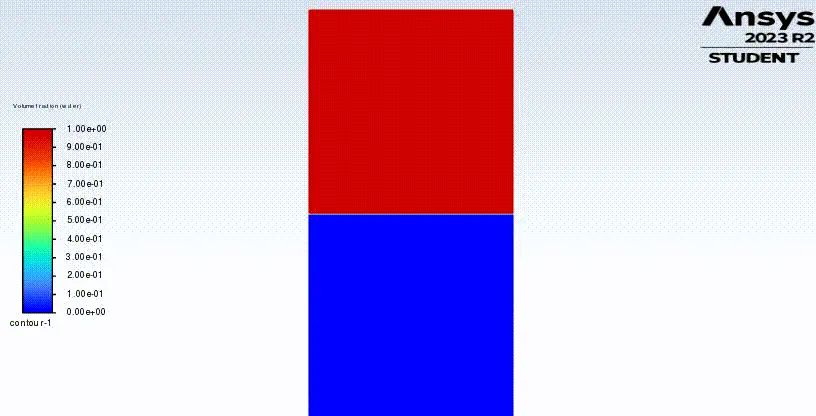
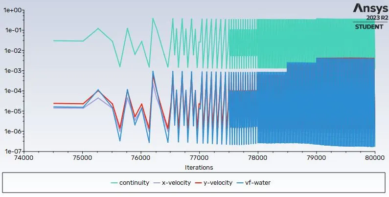
 FINE MESH (80k elements) using water and user defined material (properties listed earlier) was run for 4000 timesteps with each timestep measuring 0.001 seconds. This generated an animation of the RTI phenomenon of 4 seconds. The same can be viewed by clicking on the google drive link provided below.

Scaled residuals

Solution animation

 https://drive.google.com/file/d/1S2wh8Avbrb8vOIavXzUcvhR2ltSybZn2/view?usp=sharing

 

Atwood number (A) comparision

A = (ρ₁-ρ₂)/(ρ₁+ρ₂)

Where, ρ₁ = density of Heavier Fluid            ρ₂ = density of lighter fluid

For water-air RTI, A= (998.2-1.225)/(998.2+1.225) = 0.9975

For water-user material RTI, A= (998.2-400)/(998.2+400) = 0.4278

If we compare the 2 simulations done using fine mesh, we'll find that the fluid combination with higher Atwood number has a comparatively short-lived RTI. Whereas, the fluid combination with lower Atwood number demonstrates slightly prolonged RTI. Also, the fluid interface took more time to breach in case of fluid combination having lower Atwood number.

CONCLUSION

• Rayleigh Taylor Instability phenomena were successfully simulated.
• For base mesh, computation time was lesser, which is why 7.5 seconds of RTI could be easily simulated.
• For fine mesh, computation time was significantly higher, which is why only 4 seconds of RTI could be simulated.
• Atwood numbers were calculated and compared. Lower the Atwood number, slower the RTI phenomenon.
• Steady state solver would not be able to capture the intricate movements of the different particles as these movements are heavily dependent on time. Hence, transient solver was used.