Week 4 - CHT Analysis on Exhaust port

1. Give a brief description of why and where a CHT analysis is used.

Conjugate heat transfer (CHT) corresponds with the combination of heat transfer in solids and heat transfer in fluids. In solids, conduction often dominates whereas in fluids, convection usually dominates. CHT analysis allows for the simulation of heat transfer between solid and fluid domains by exchanging thermal energy at the interfaces between them. CHT analysis can accurately predict heat transfer by simultaneously solving all the relevant solid and flow field heat transfer processes. It has benefits for those applications where heat transfer is either non-uniform or difficult to calculate empirically. Typical applications of this analysis type are, simulation of heat exchangers, cooling of electronic equipment, industrial machinery, powerplant exhaust systems, etc.

AIM

To simulate hot air flow through a multiport exhaust channel and analyse the conjugate heat transfer of the simulation.

OBJECTIVES

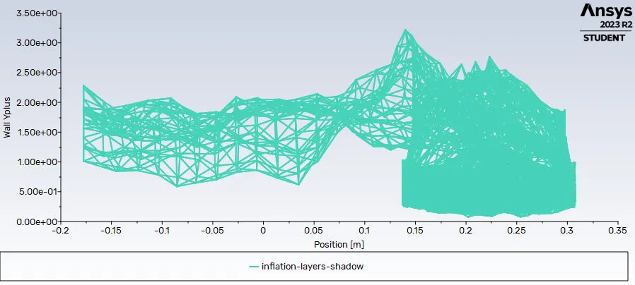
• Maintain the y+ value according to the turbulence model and justify the results.
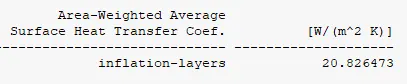
• Calculate the wall/surface heat transfer coefficient on the internal solid surface & show the velocity & temperature contours in appropriate areas.

PRE-PROCESSING

GEOMETRY 

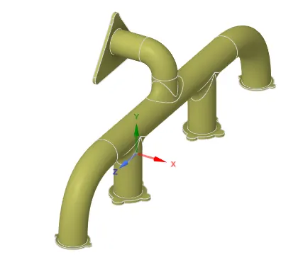
The multiport exhaust model geometry was imported to SpaceClaim and fluid fluid volume was created inside the solid volume using volume extraction tool.

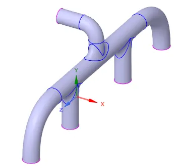
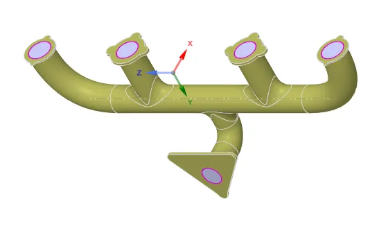
After that the new components were moved to a new folder and the topology was shared across both solid and fluid volumes.

 

MESHING

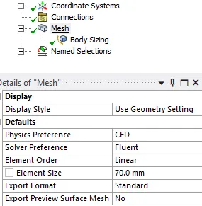
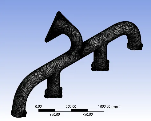
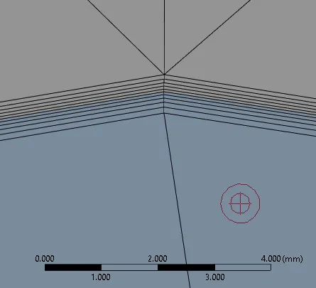
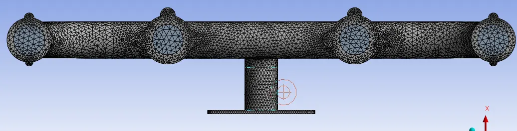
First a base mesh was generated to ensure unflawed geometry. Then, named selections were entered to distinguish the surfaces and bodies. After that 5 inflation layers on each side were provided at the contact surface between the solid and fluid volumes. The first layer thickness was adjusted by hit and trial and finally kept at 0.05 mm because it ensured an average y+ value less than 1. This was necessary to ensure that the k-omega SST turbulence model will be able to capture the heat transfers near the wall correctly. The mesh element size was decreased to 70 mm to capture the flow physics better. Finally, a body sizing of 10 mm was applied to the solid volume to improve the simulation (Curve capture was set to YES). All these generated a mesh with 0.4 million elements which is solvable using student license.

   

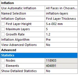
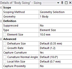
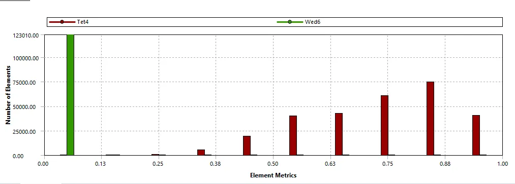
Following snapshots show the zoomed inflation layers and the obtained mesh.

 

SOLVER

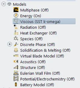
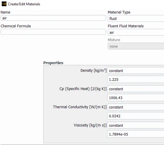
Pressure-based and Steady state solver was used to simulate the flow. Energy equation was turned ON. K-Ω SST turbulence model was applied. Cell zone conditions were checked. Solid volume used aluminium and fluid vloume used air as material with default properties as shown below.

 

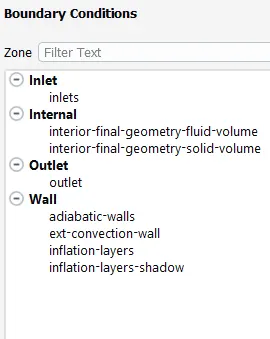
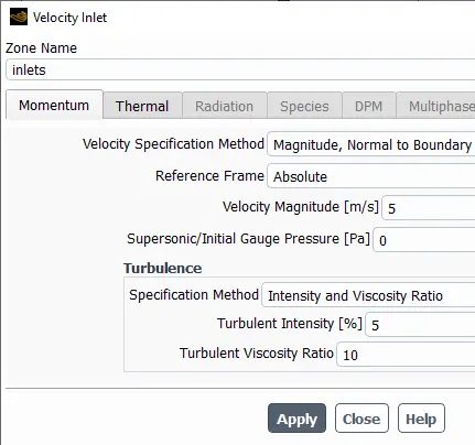
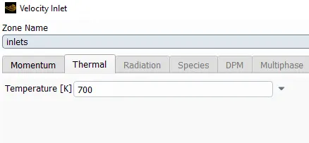
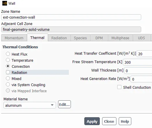
Boundary Conditions: 5 m/s velocity and 700 K temperature were applied to inlet; 20 W/m²K HTC was applied to external convection wall; and rest named selections were kept as wall with no-slip.

  

Solution method: Coupled solution method was used since it takes less time to compute.

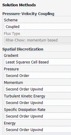
The process was hybrid initialised and run for 500 iterations.

RESULTS

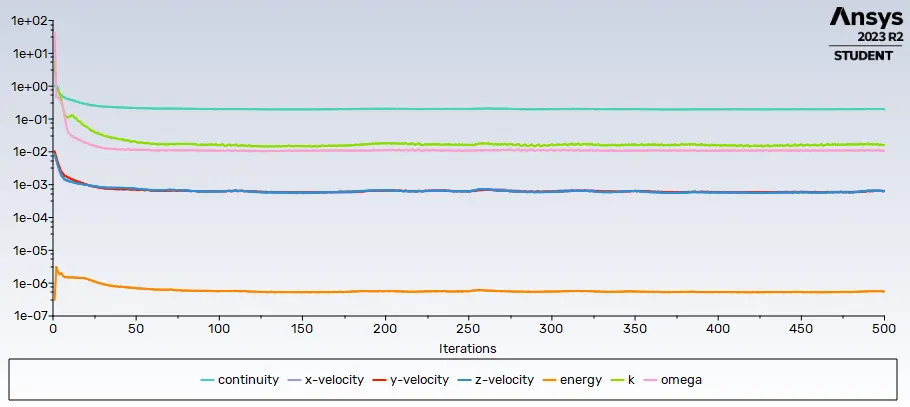
Scaled Residuals

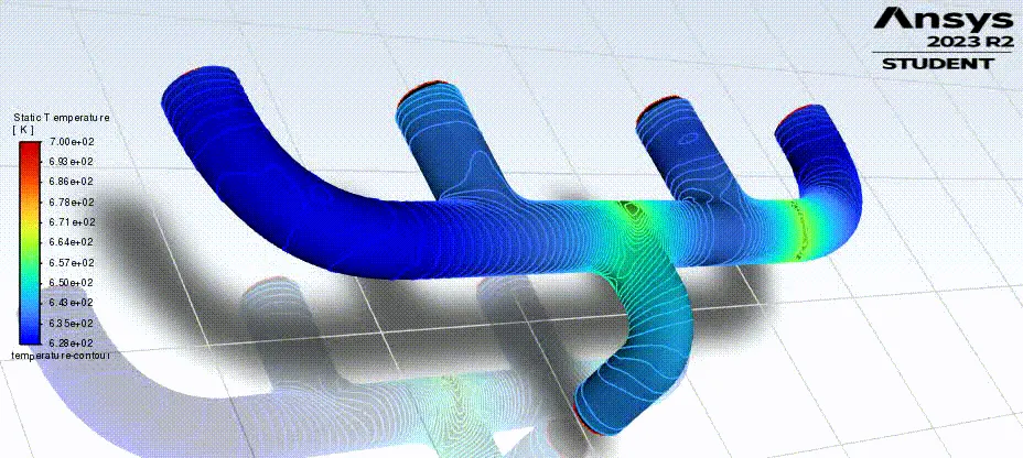
Solution Animation of temperature contour

Y+ values were maintained at y+<1>

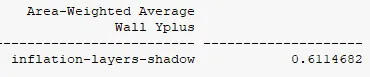
To calculate the area-weighted average of wall Y+ and later on surface HTC, the surface integral tool of Fluent was used. It is available under the Reports tab. In surface integral, we can choose wall y+ under turbulence section. Similarly, for surface HTC we can choose the same under Wall Fluxes.

To obtain a wall y+ value plot as shown below, we have to use the XY-plot tool under Results tab.

Surface heat transfer coefficient at internal solid surface was calculated using Surface Integral and had an average value of 20.8 W/m²K, which is close to the bounadry condition we provided for external convection wall.

 

POST-PROCESSING

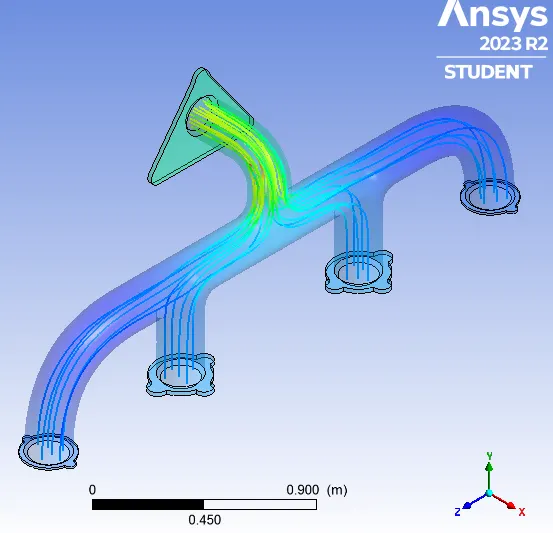
Below given snapshot showcases the temperature variation along the external convection layer alongwith the streamlines showing the path of the fluid particles.

 

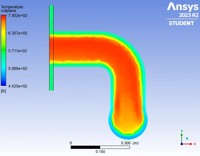
A cut plane was created dissecting the outlet channel longitudinally.

Temperature contour at cutplane:

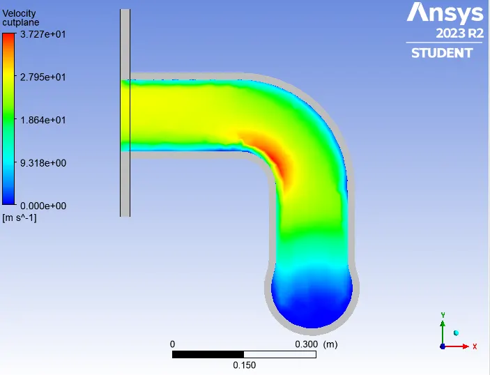
Velocity contour at cutplane:

Surface HTC at cutplane alongwith velocity vectors:

 

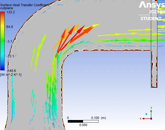
 We had observed earlier from the velocity contour that the inner section of bending witnesses highest velocity of exhaust air. Again, in the above picture we see the vectors showing the same thing. Also, the surface HTC near that section seems to be high. The high velocity causes faster transfer of heat energy from the fluid to the solid wall, thus increasing the HTC of that surface.

 CONCLUSION

• CHT analysis on exhaust port was simulated successfully using ANSYS Fluent.
• An adequately fine mesh was obtained using inflation and body sizing tools.
• The velocity at outlet is higher than inlet. This shows conservation of continuity, since, there are 4 inlets but only 1 outlet of equal cross-sections of area.
• Y+ value was mantained below 1, thus meeting required criteria for k-omega turbulence model to run successfully.
• Average Surface HTC obtained after solving was 20.8 W/m²K for the inner portion of solid volume.
• The velocity near the wall at inlet is very close to 0, which shows the presence of boundary layer and the activation of no-slip phenomenon.