Week 5 - Rayleigh Taylor Instability
- What are some practical CFD models that have been based on the mathematical analysis of Rayleigh Taylor waves? In your own words, explain how these mathematical models have been adapted for CFD calculations.
Rayleigh-Taylor (RT) instability is a fluid dynamics phenomenon that occurs at the interface between two fluids of different densities when the lighter fluid is accelerated into the denser fluid under the influence of gravity. This instability leads to the formation of complex, nonlinear structures known as Rayleigh-Taylor waves. Computational Fluid Dynamics (CFD) models based on the mathematical analysis of Rayleigh-Taylor waves have been developed to simulate and predict the behavior of these waves in various practical scenarios.
Some practical CFD models that incorporate Rayleigh-Taylor wave analysis include:
1. Level-Set Methods: Level-set methods are commonly used in CFD simulations to track and capture interfaces between different fluids. These methods use a scalar function (the level-set function) to represent the position of the interface. For Rayleigh-Taylor simulations, this approach can be adapted by solving the Navier-Stokes equations along with the level-set equation to model the evolution of the interface between the fluids.
2. Volume of Fluid (VOF) Methods: VOF methods are another approach to simulate fluid interfaces. In this method, the domain is divided into cells, and the fraction of each cell occupied by a particular fluid phase is tracked. This allows for accurate representation of the evolving interface between fluids with different densities, making it suitable for Rayleigh-Taylor simulations.
3. Implicit Large Eddy Simulation (ILES)**: ILES combines the benefits of Large Eddy Simulation (LES) with implicit time integration schemes. LES resolves large-scale turbulent structures while modeling smaller scales. In Rayleigh-Taylor simulations, ILES can capture the complex turbulent flow patterns that develop at the interface between the two fluids.
4. High-Resolution Shock-Capturing Scheme: These schemes are used to solve hyperbolic conservation laws, such as the Navier-Stokes equations. They are well-suited for simulating shock waves and discontinuities in fluid flows. When adapted for Rayleigh-Taylor simulations, these schemes can handle the sharp density gradients and shock-like features that emerge in the mixing zones.
The adaptation of mathematical models for Rayleigh-Taylor waves into CFD calculations involves solving the fundamental equations of fluid motion (Navier-Stokes equations) along with additional transport equations or methods specifically designed to track the interface between the two fluids. The process generally involves the following steps:
1. Numerical Discretization: The continuous partial differential equations governing fluid flow are discretized into a finite volume or finite difference framework, allowing for numerical simulation on a discrete grid.
2. Interface Tracking : The chosen method (e.g., level-set or VOF) is used to track the evolving interface between the fluids as it deforms due to the Rayleigh-Taylor instability.
3. **Turbulence Modeling**: Depending on the scale of the simulation and the desired accuracy, various turbulence models may be employed to capture the effects of turbulence and mixing at the interface.
4. Boundary Conditions- Appropriate boundary conditions are applied at the walls and outer boundaries of the simulation domain to mimic real-world conditions and interactions.
5. Time Integration: Time-stepping algorithms are used to advance the simulation in time, capturing the dynamic evolution of the Rayleigh-Taylor waves.
6. Visualization and Analysis**: Post-processing tools are employed to analyze and visualize the simulation results, allowing researchers and engineers to gain insights into the complex fluid behaviors and structures arising from the Rayleigh-Taylor instability.
In summary, CFD models based on the mathematical analysis of Rayleigh-Taylor waves involve adapting numerical methods to accurately simulate the evolution of fluid interfaces, turbulence, and mixing driven by the instability. These models find applications in various fields, including astrophysics, engineering, and materials science, where Rayleigh-Taylor instabilities play a significant role.
2. Perform the Rayleigh Taylor instability simulation for 2 different mesh sizes with the base mesh being 0.5 mm. Compare the results by showing the animations( Attach them from your google drive). Observe the differences in the animation and explain the effect of mesh size on simulation. Also, explain why a steady-state approach might not be suitable for these types of simulation.[ Choose Air and Water for this simulation]
Here the dense fluid is on top and lighter fluid is at the bottom.Thier Interface becomes unstable in the presence of gravity.
We are learning Volume of Fluid method in this course,which is an important technique used in two phase flows.
Type of Analysis - 2D
1. Baseline Setup-
Geometry Setup - Spaceclaim
Creating 20 x 20 square and using Pull tool to create a surface, same process is repeated to form one more square with same dimensions.
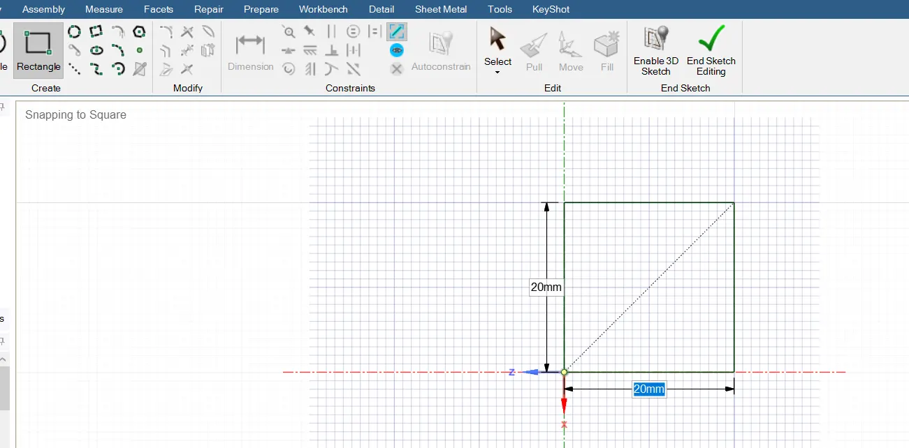
Two new components are named as air and water , each sqaure at each component.
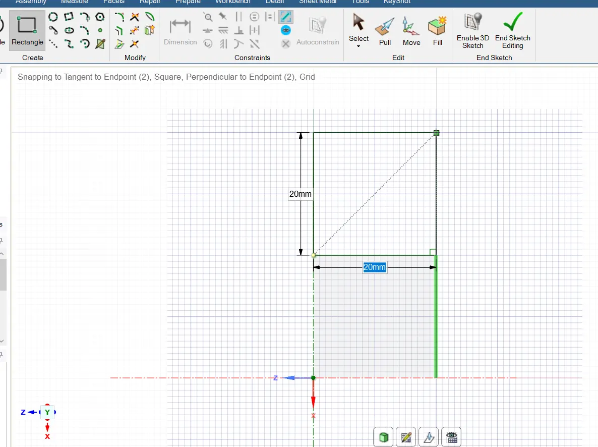
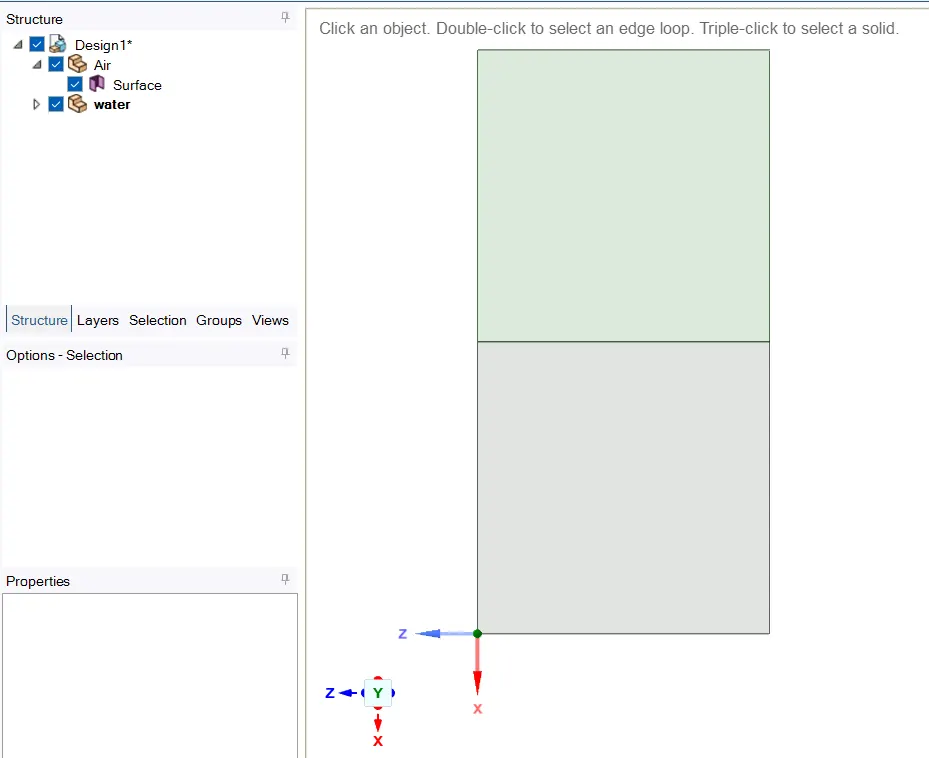
To form a conformal mesh, faces must be rightly shared.
Workbench - Share- select both components, one edge which is being shared turns blue.
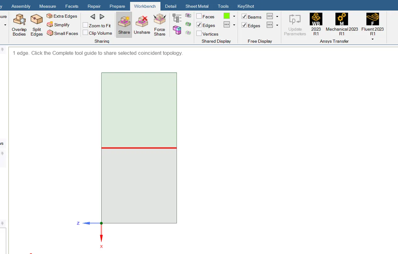
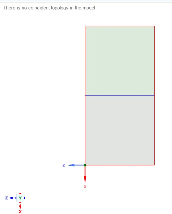
Share Topology - Share - which is enabled automatically.
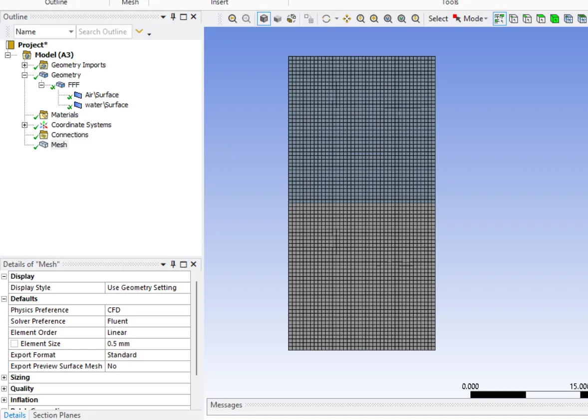
Mesh Setup
Mesh Size - 0.5 mm
Fluent Setup
Pressure Based , Transient Simulation
Gravity Enabled at negative Y direction
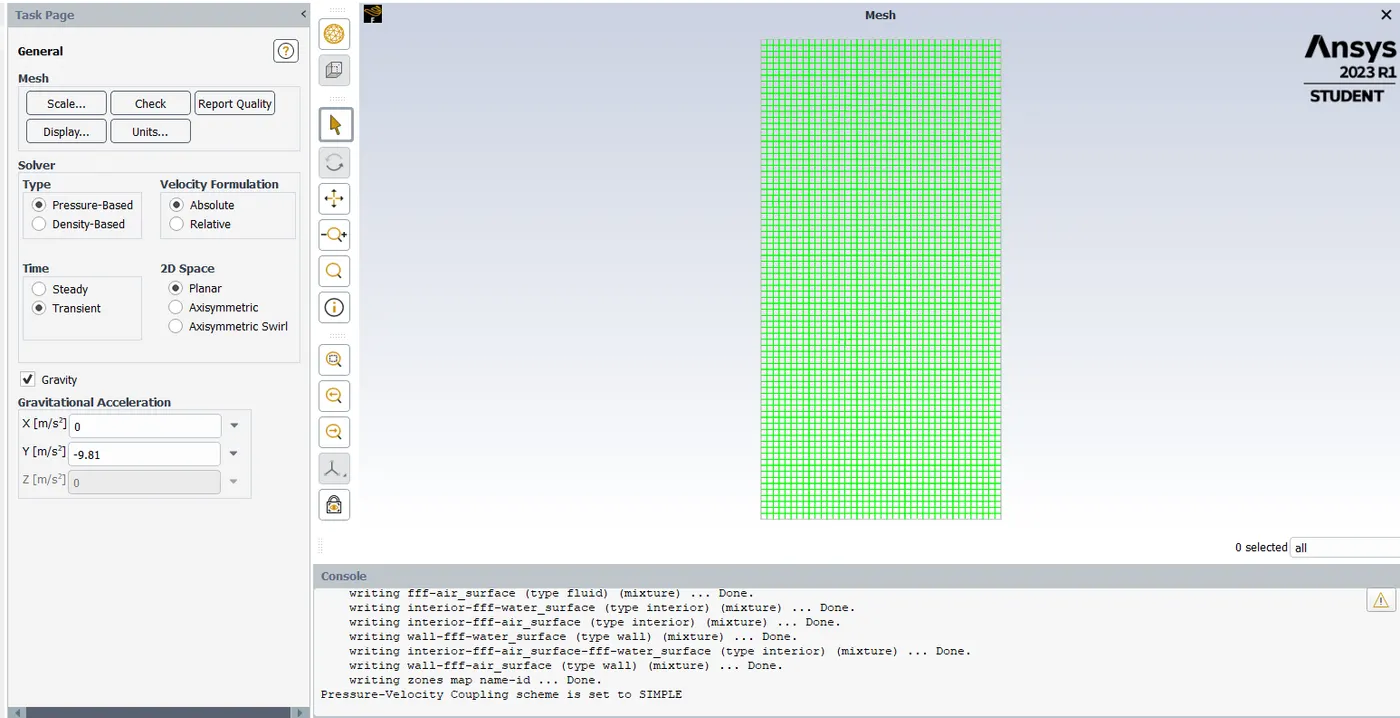
we do not need Energy Equation , Turbulenece Model - Laminar
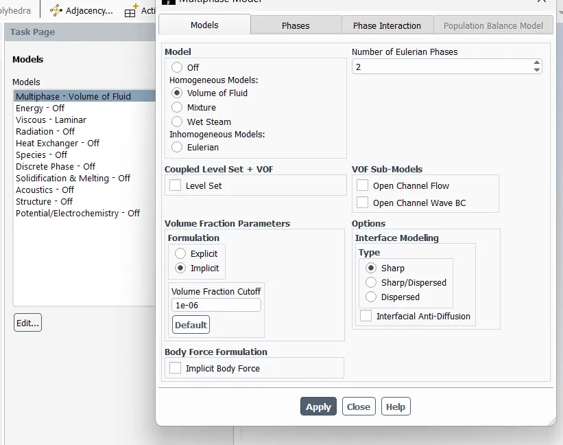
Enable Multiphase Model - Volume of fluid
No. of phases - 2
Implicit Method
Adding 'water' as material from fluent database in Materials
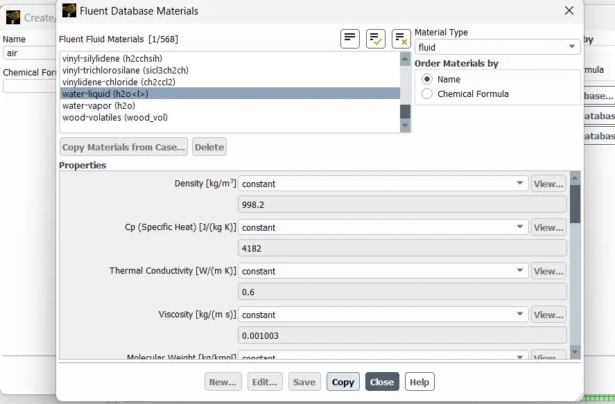
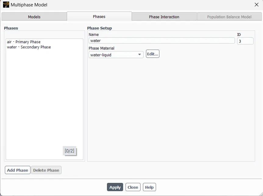
List Phases
Assigning Primary and Secondary Phases
Check Zones of Water and Air
Water zone should be above of air zone.
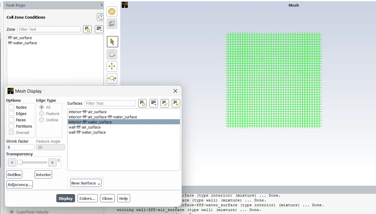
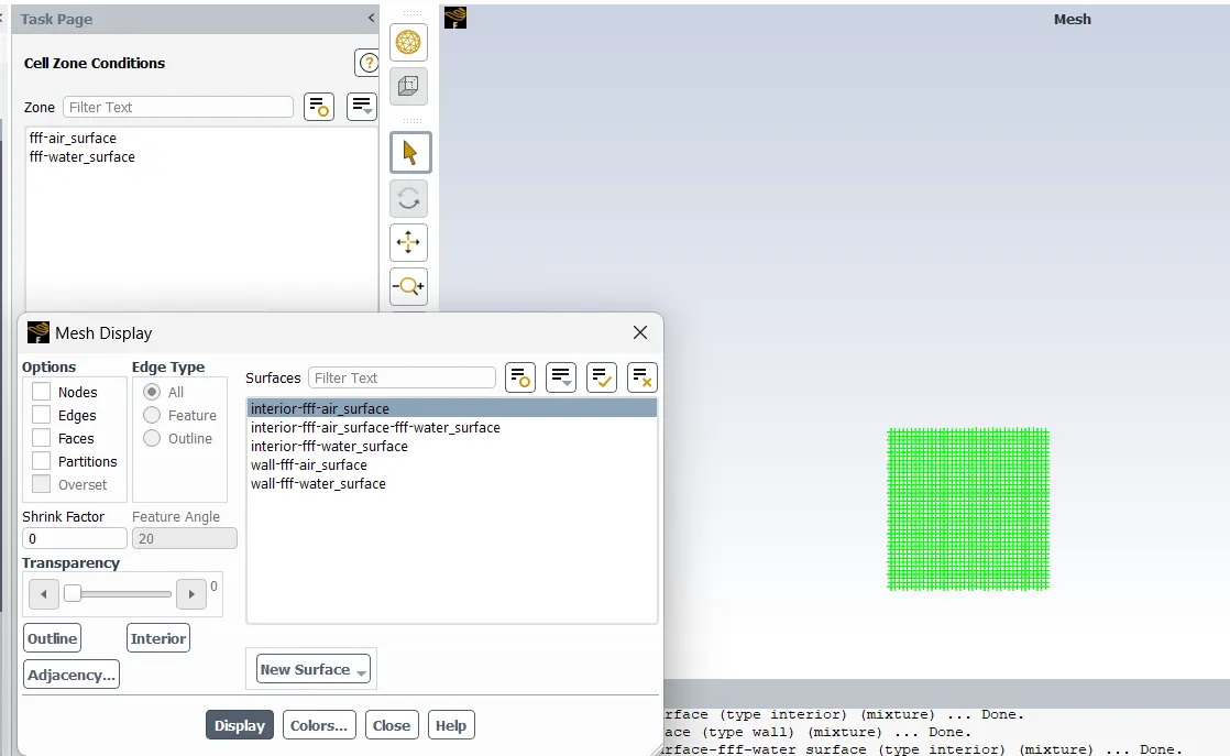
Standard Initialization
Patch
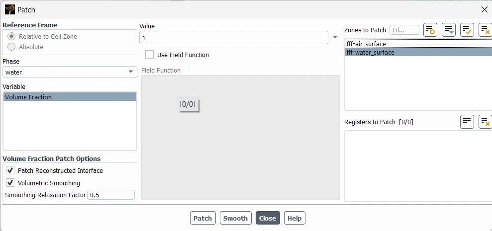
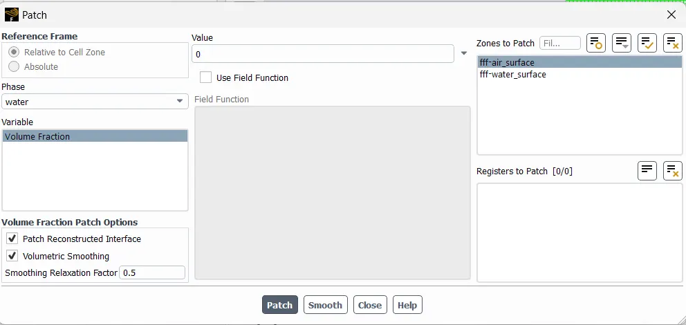
Time Step Size - 0.05 s
No. of Time Steps- 1500
Display - Contours
Phases - Volume of Fraction
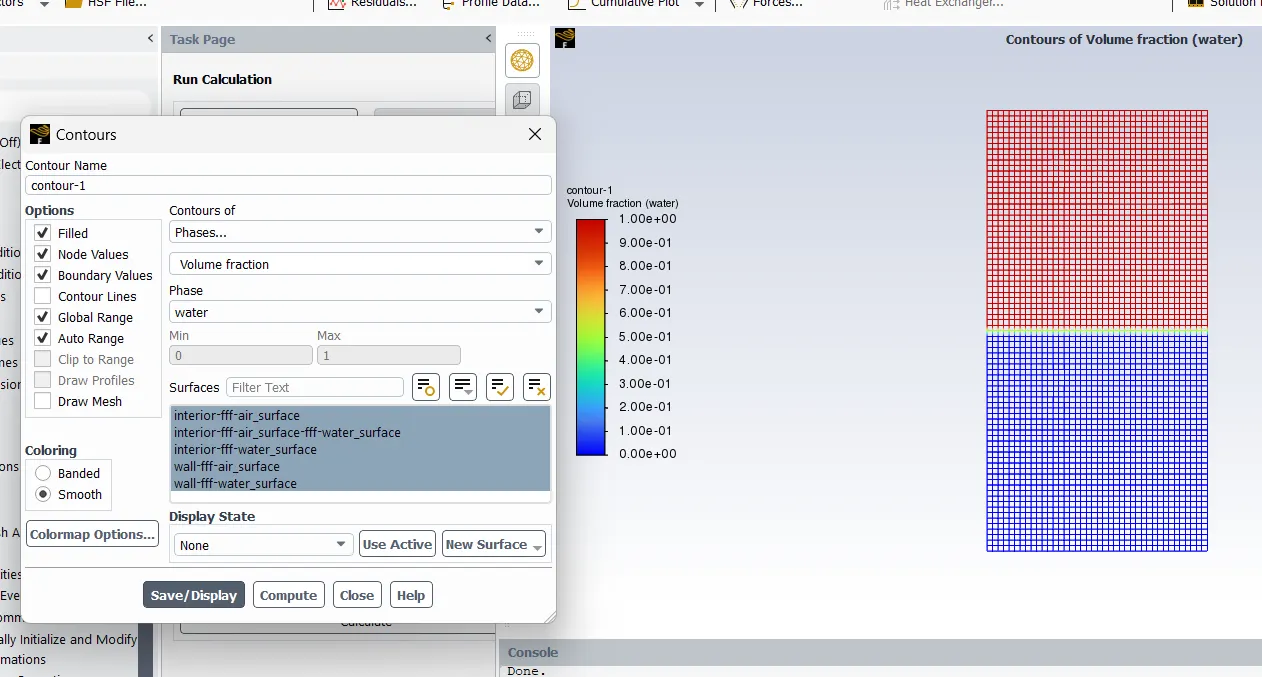
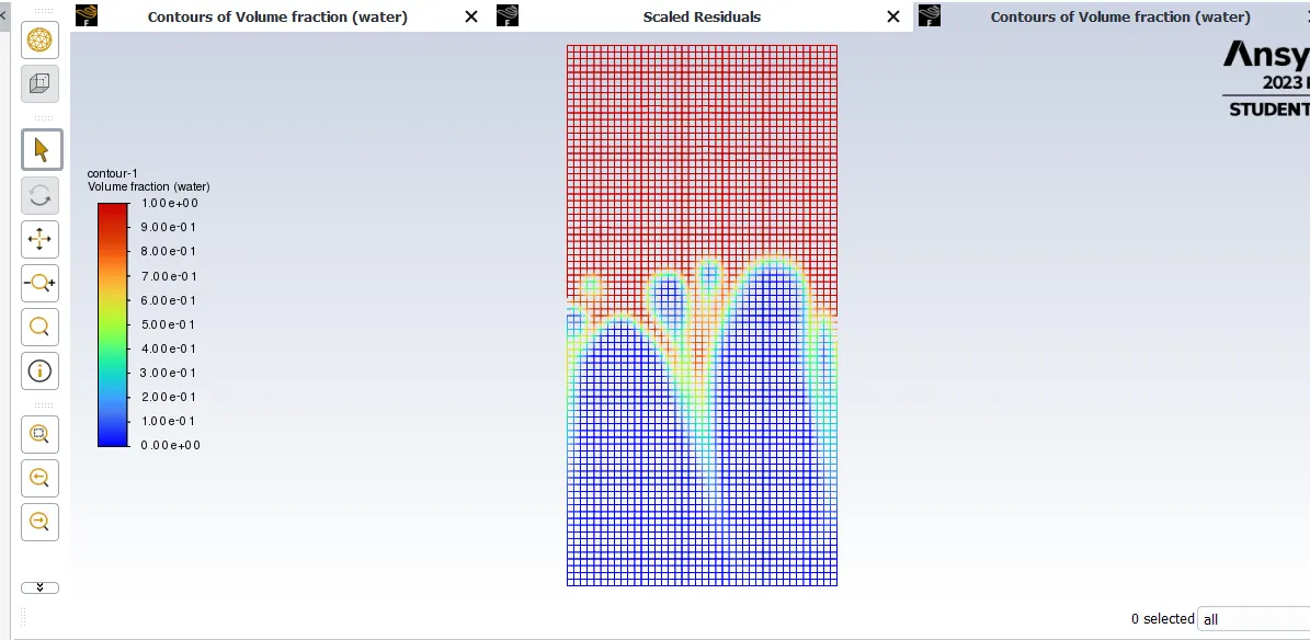
Bubble like structure is seen, which we call as Rayleigh Taylor Instability
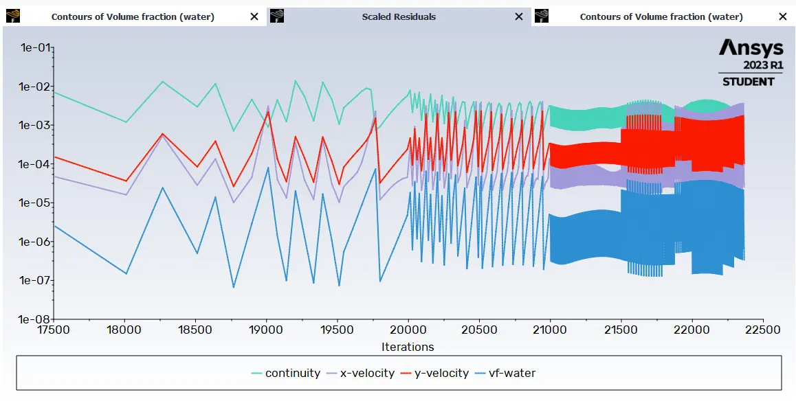
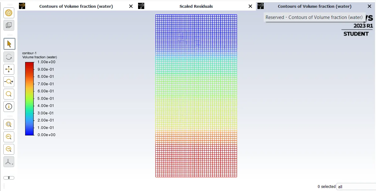
Animation Link - https://drive.google.com/file/d/1YuMH1visIyHgq5cvuPmwdOPC-G0li_YF/view?usp=sharing
2. Refined Mesh - Case 1
Mesh Size - 0.4 mm
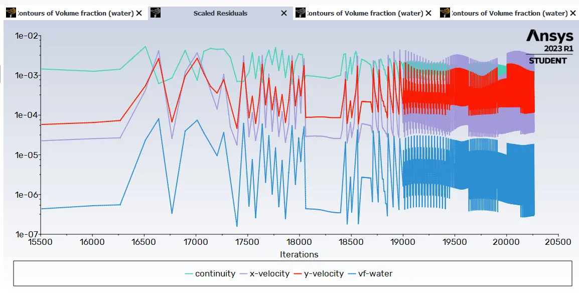
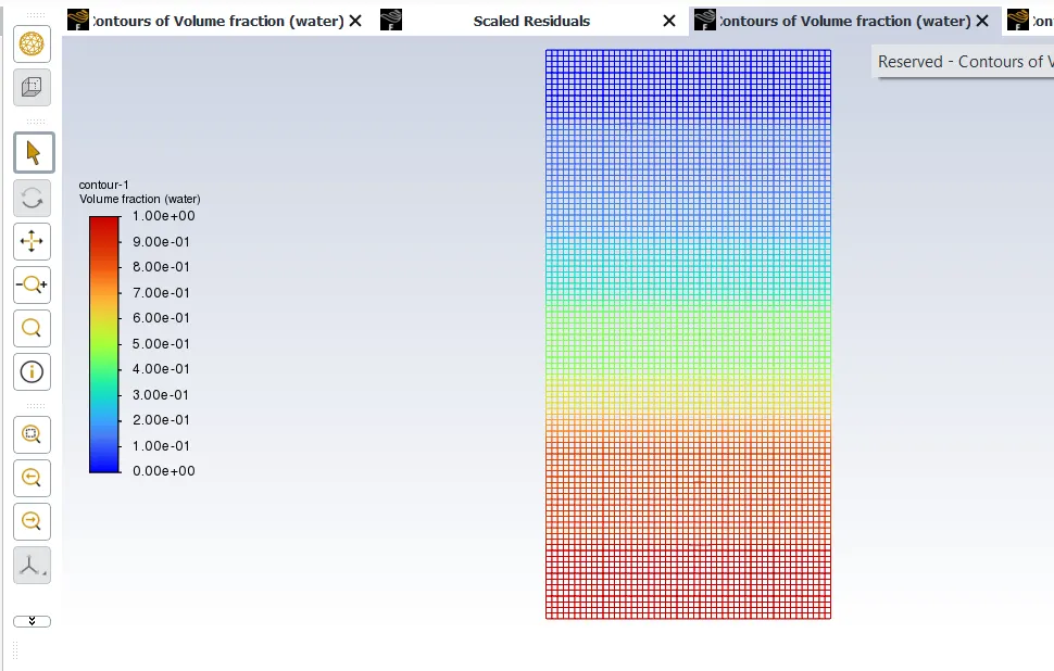
Animation Link - https://drive.google.com/file/d/1YuMH1visIyHgq5cvuPmwdOPC-G0li_YF/view?usp=sharing
2. Refined Mesh - Case 2
Mesh Size - 0.2 mm
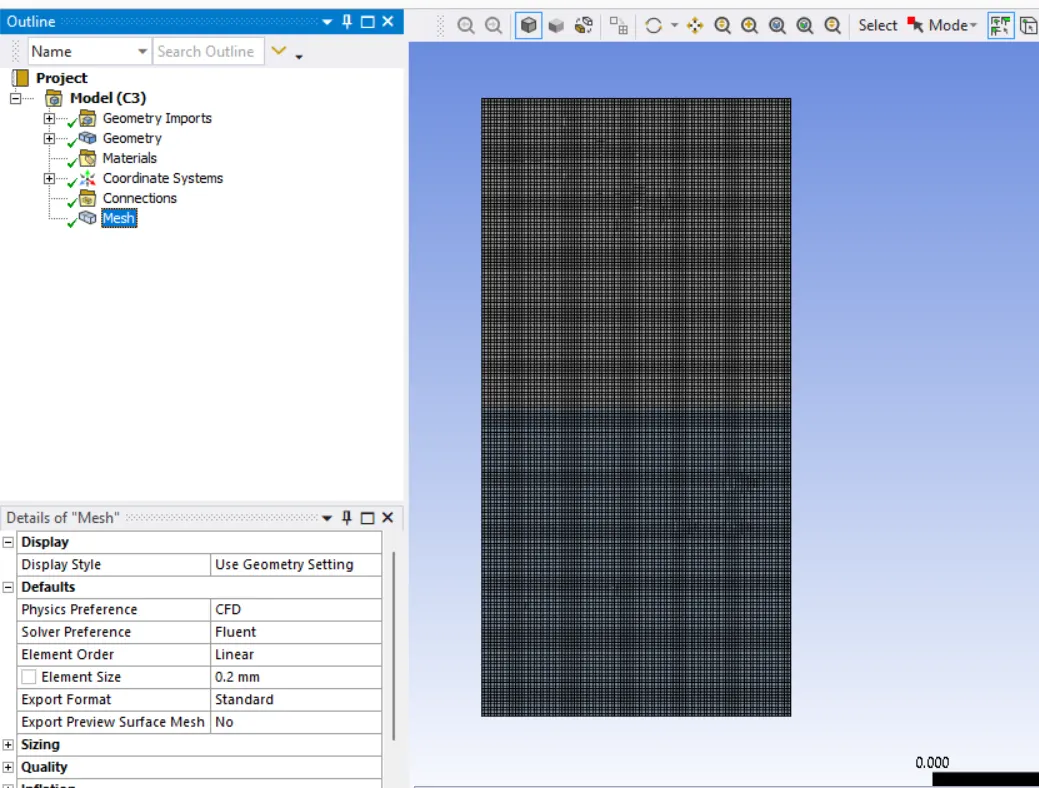
Animation Link - https://drive.google.com/file/d/1JAPU470clUrpayoGIpqs3SttH0dztjXm/view?usp=sharing
Conclusion
- 1.As the mesh is finer, we are able to capture the instability more precisely.
- 2. No. of colour patterns are more when mesh size is increased, which shows the mixture value correctly.
- 3. The Instability phenomenon occurs with respect of time and time factor is not considered in steady state simulation. hence steady state approach is not suitable.
3. Run one more simulation with water and user-defined material(density = 400 kg/m3, viscosity = 0.001 kg/m-s) for refined mesh.
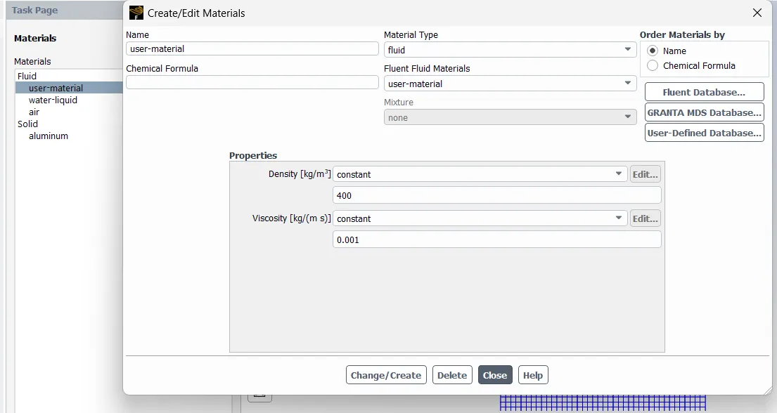
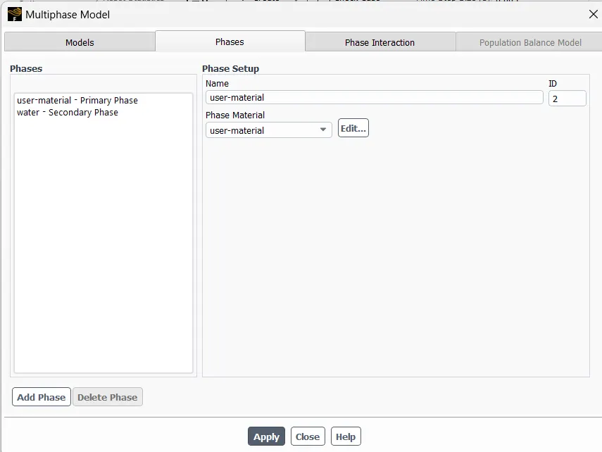
As the density of water is greater, it must be on the top.
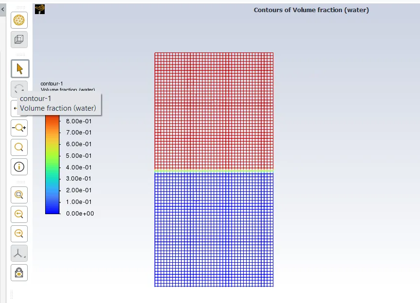
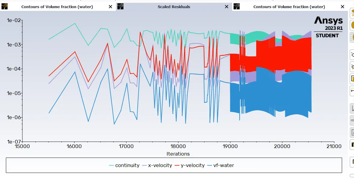
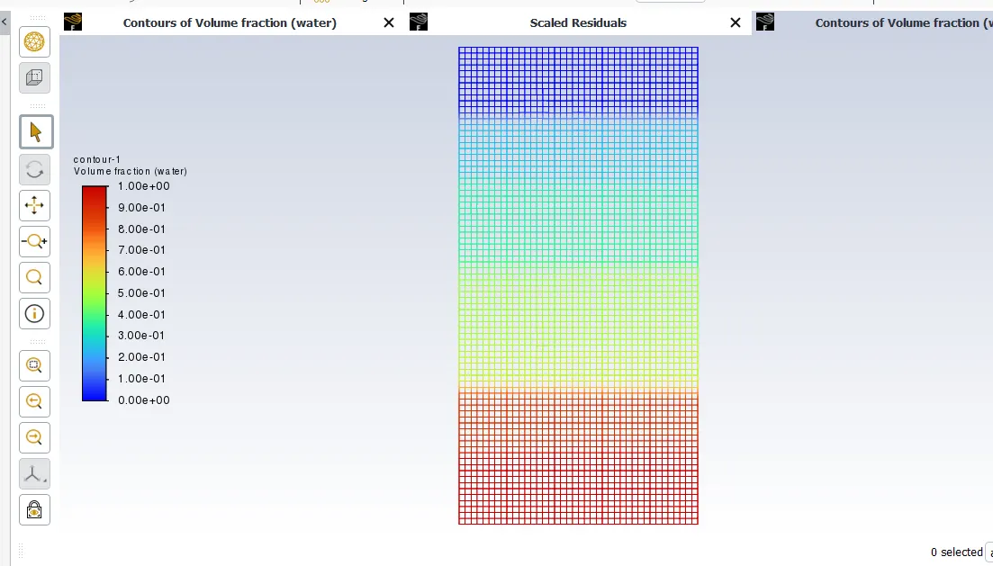
Animation Link - https://drive.google.com/file/d/1EKmWdha8i0OEyZ4BHP8b4NyffNMPpirR/view?usp=drive_link
4. Define the Atwood Number. Find out the Atwood number for both the cases and explain how the variation in Atwood number in the above two cases affects the behavior of the instability.
The Atwood number, often denoted as "A" or "At," is a dimensionless parameter used in fluid dynamics and fluid mechanics to describe the behavior of fluids in a gravitational field when there is a density difference between two immiscible fluids. It specifically relates to the motion and stability of interfaces between these fluids.
Mathematically, the Atwood number is defined as the absolute value of the difference in densities of the two fluids divided by the average density, all multiplied by the acceleration due to gravity:
At = ρ1 - ρ2 / ρ1 + ρ2
Where:
- ρ1 and ρ2 are the densities of the two fluids.
The Atwood number quantifies the importance of buoyancy forces relative to inertial forces in the fluid system. When the Atwood number is close to 0, the two fluids have similar densities, and the buoyant effects are negligible. However, as the Atwood number deviates from 0, the density difference between the fluids becomes more significant, leading to distinct flow behaviors, such as interfacial instabilities, mixing, and overturning.
In various fluid dynamic applications, such as the study of Rayleigh-Taylor instability (which occurs when a denser fluid is placed above a lighter fluid), the Atwood number plays a crucial role in predicting the growth of instabilities and the subsequent fluid motion. It helps researchers and engineers understand how gravitational forces interact with density differences to influence the fluid's behavior
1. Atwood Number in First Case ( Air and Water)
ρ1 - 998.2 kg/m^3
ρ2 - 1.225 kg/m^3
Atwood Number = { ρ1 - ρ2 / ( ρ1 + ρ2) ] = { 998.2 - 1.225} / ( 998.2 +1.225 ) } = 996.975/ 999.425 = 0.99
Here At = 0.99, which is close to 1, that means here the density difference between two fluids is significant.
Positive Value shows that the heavier fluid is on the top.
2. Atwood Number in First Case ( User Defined Material and Water)
ρ1 - 998.2 kg/m^3
ρ2 - 400 kg/m^3
Atwood Number = { ρ1 - ρ2 / ( ρ1 + ρ2) ] = { 998.2 - 400 } / ( 998.2 +400 ) } = 598.2 / 1,398.2 = 0.43
Here value is less than 1 and the previous case. Here difference between densities is less than the first case.
Turbulence and shocks will be less significant.