Week 2 - Flow over a Cylinder.
Introduction
Vortex Sheding
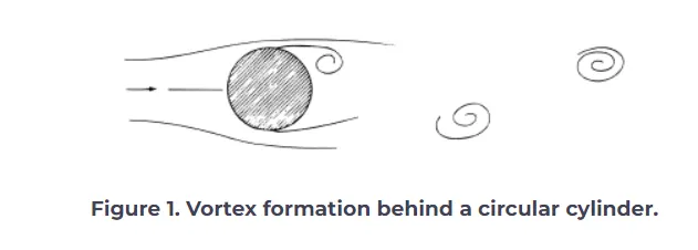
An oscillating flow is formed when a fluid flows over an object. Vortices are formed behind the body, In our case it is a cylinder. The fluid flow over the object forms alternating low-pressure vortices on the downstream side of the object. The object will move to the low-pressure zone.
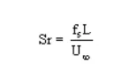
Strouhal number Sr , is a dimensionless quantity which is used to measure frequency of shedding.
Flow Over Cylinder
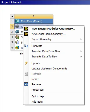
On Ansys Workbrnch , a Fluid Flow system is launched and named as ' Flow Over Cylinder'
Geometry is launched using Spaceclaim
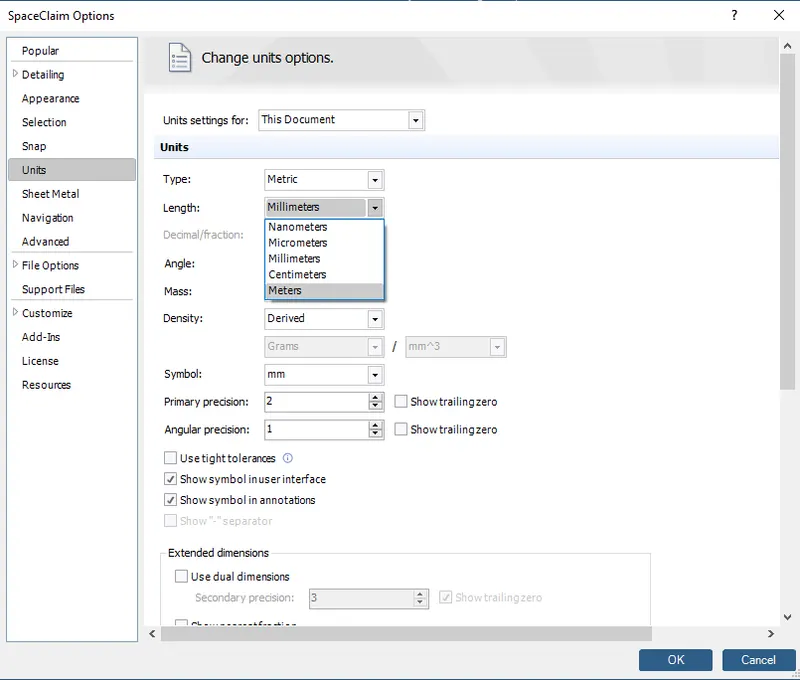
Changing Units to Meters
Drawing Circle of 2 Meters
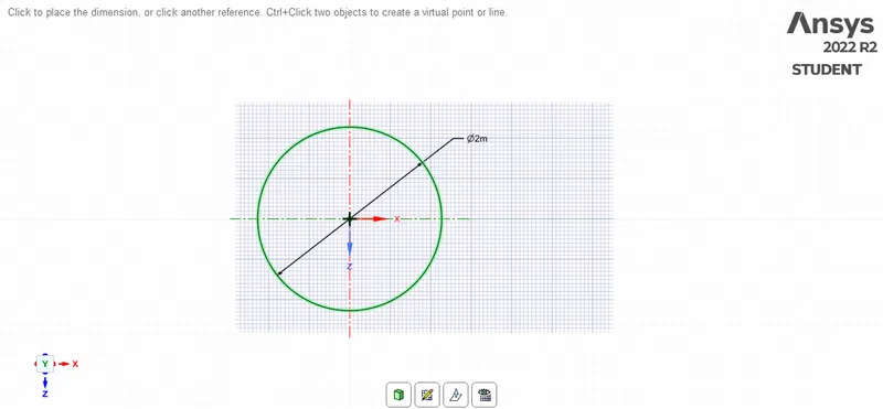
Creating Computational Domain
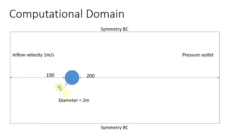
From Inlet to centre of Diameter = 10D = 20 m
From Outlet to centre of Diameter = 20D = 40 m
Total Length of Inlrt = 10 D = 20 m
A rectangle is formed using above dimensions.
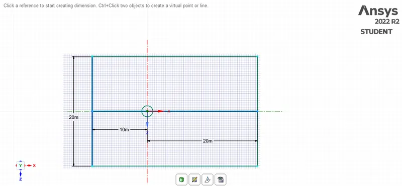
After selecting Pull Option , Geometry is converted to surface.
Selecting the circle inside and deleting it , Deleting Construction Lines
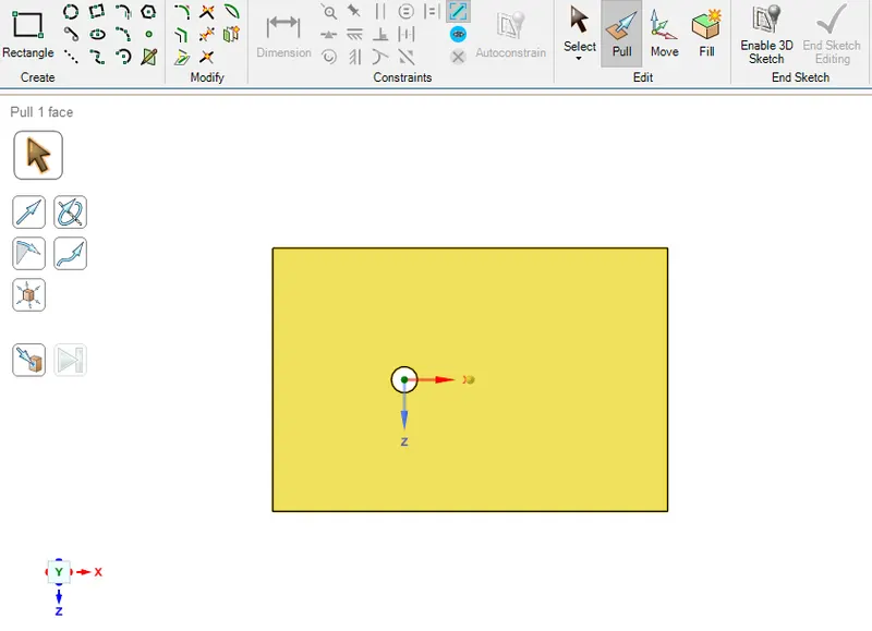
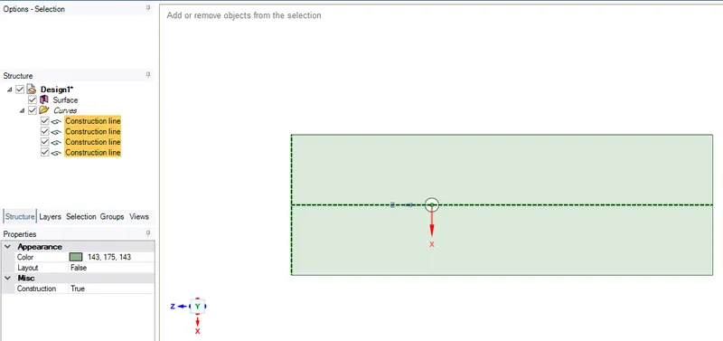
Concluding with the geometry
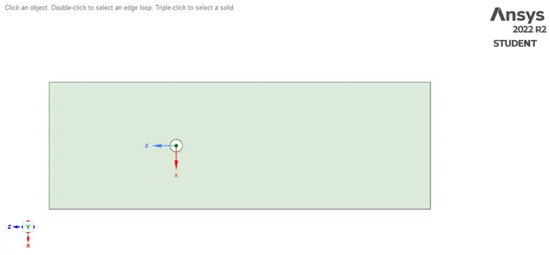
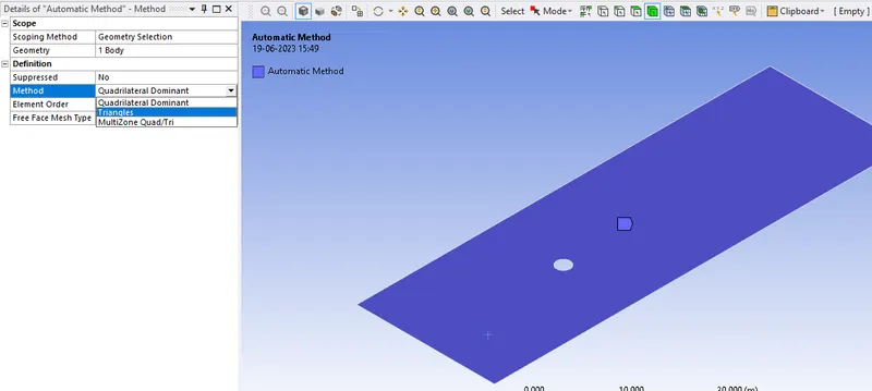
Meshing
Insert Method - Automatic Method - Triangles
Mesh - Element Size - 2 m
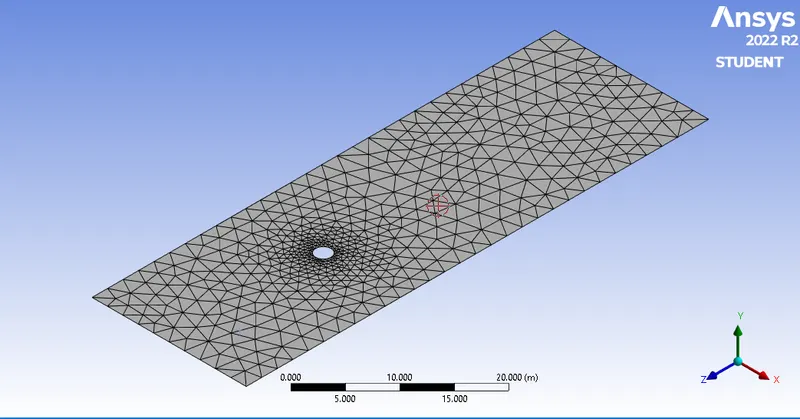
Insert Edge Sizing to generate refined mesh near circle
No. of Elements - 36
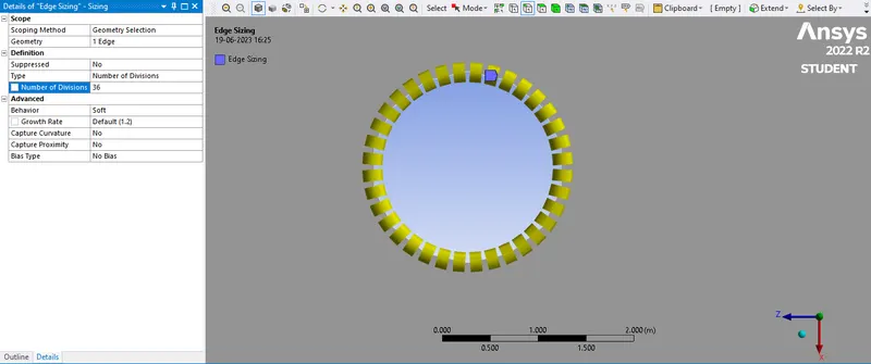
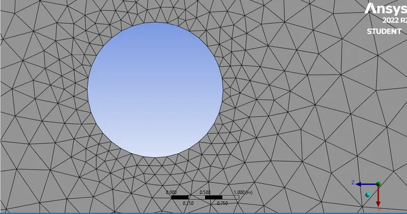
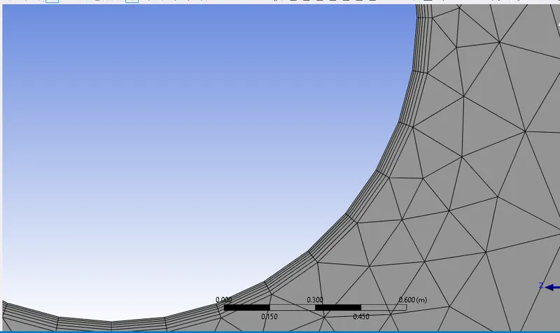
Inflation Layer helps in achieving body fitted mesh.
It helps in capturing boundry layer phenomena
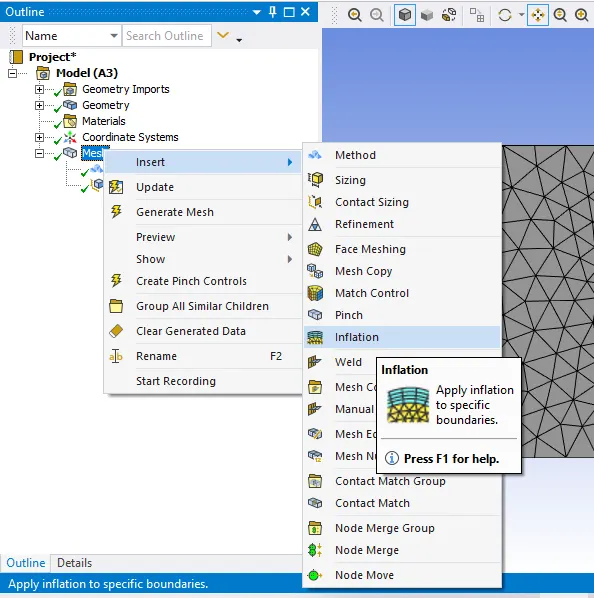
Insert - Inflation
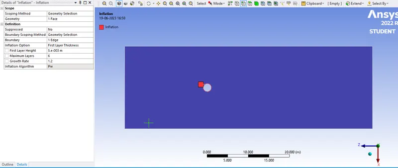
Wall is selected as a geometry and edges of a circle as boundry
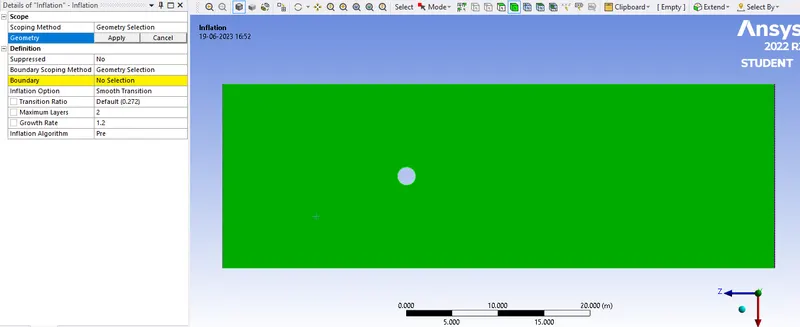
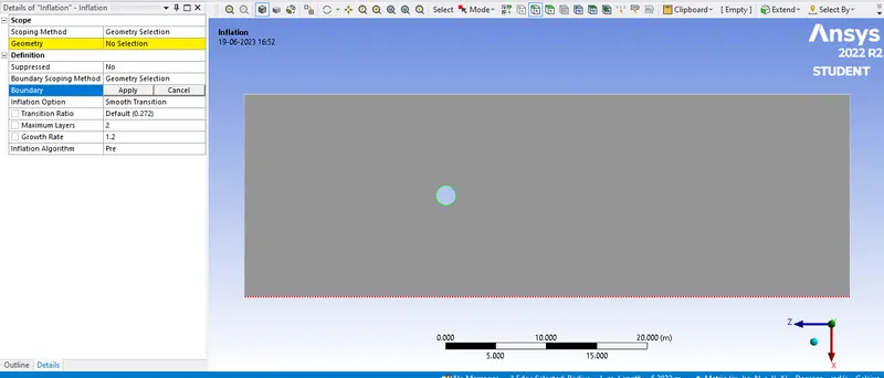
Inflation Option - First Layer Thickness , First Layer Height = 5e-3 , Maximum Layers = 6
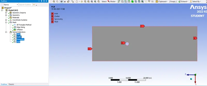
Assigning names
Fluent Setup
Steady State - Pressure Based
Viscous Model - Laminar , max. Re no. = 100, hence no turbulence will be present
Defining new user material
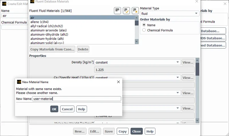
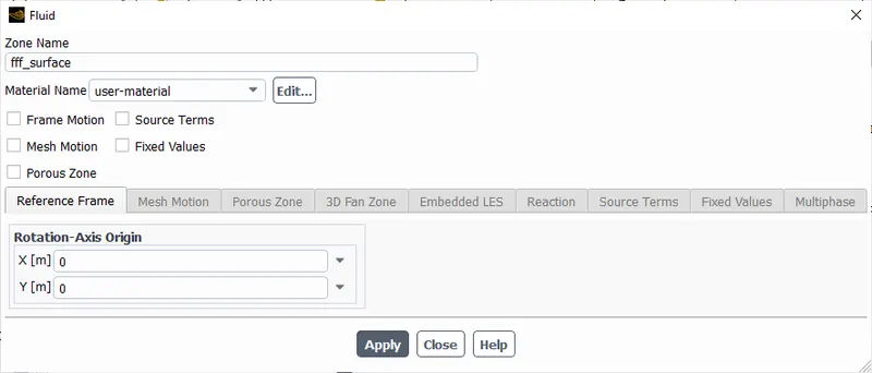
Cell zone conditions ( which define volume) - Assinged with new material
Deleting air from materials
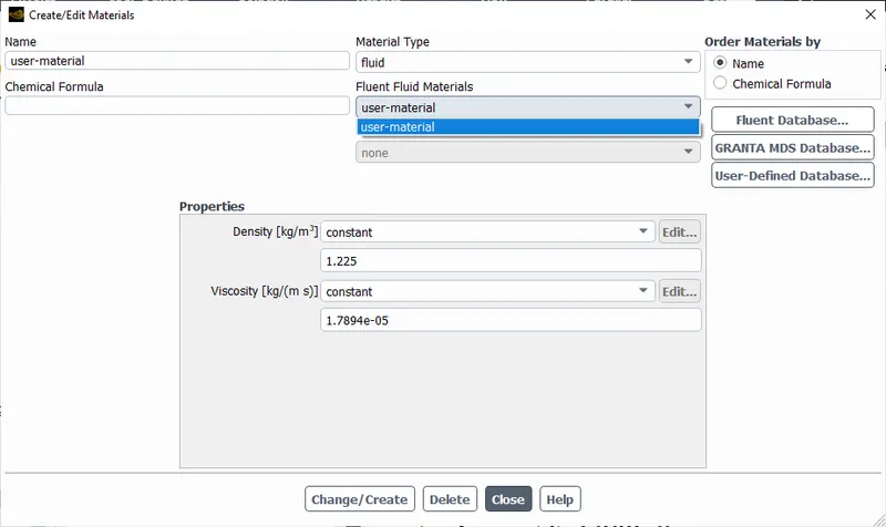
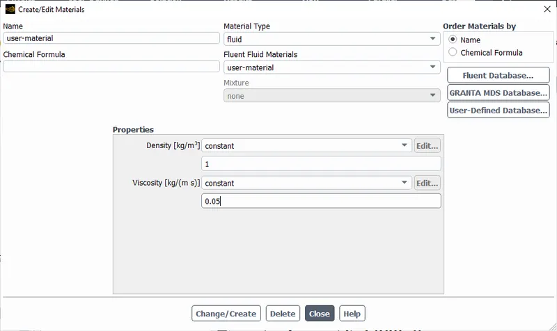
Assigning values as
Density = 1 kg/m^3 , Viscocity = 0.05 kh/m s
Because at these values a vortex shaadig phenomenon is observed even in laminar flow.
This is called as karman vortex street phenomenon
Boundry Condition
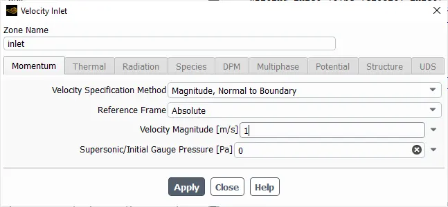
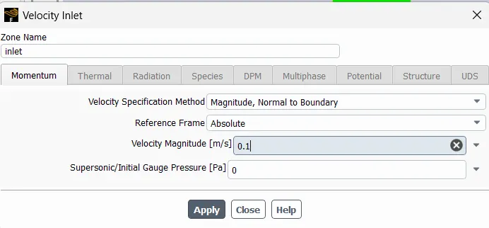
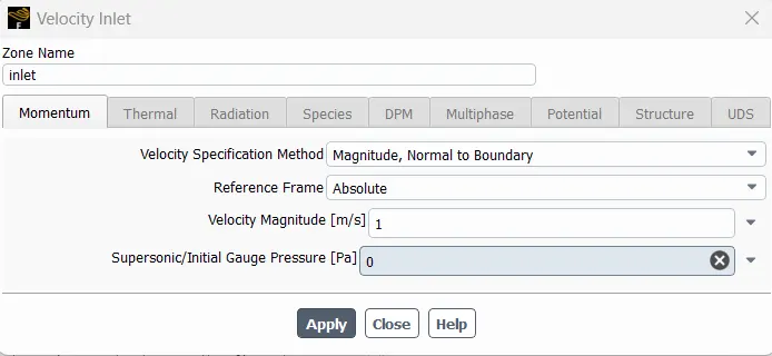
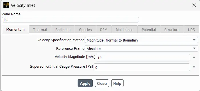
Velocity Inlet = Velocity at Inlet = 1 m/sec Guage Pressure = 0 Pa i.e 1 Atm Pressure
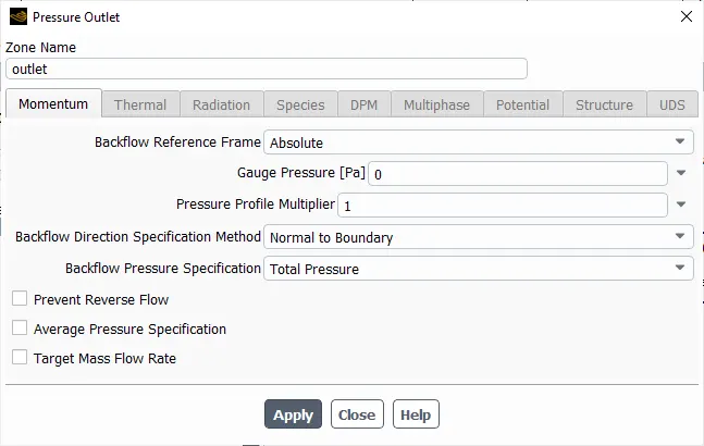
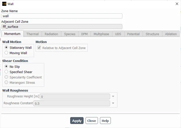
No Slip Condition at Wall
Definitions
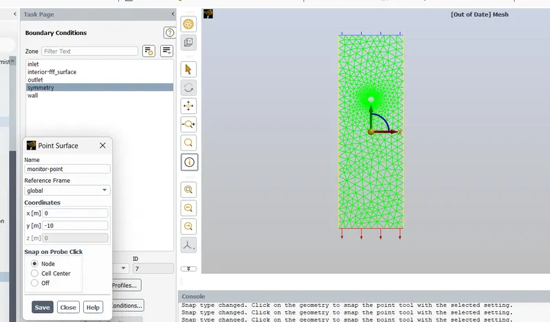
We need to create a monitor point
4*D to the right side of cylinder
Result - Point Surface - Giving Co-ordinates
Name of point - Monitor Point
Definitions - Surface Reort - Vetrex Averge - Velocity
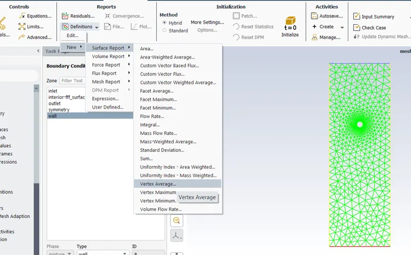
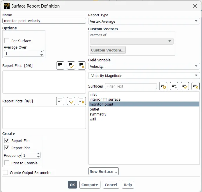
Creating Vortex Velocity Average at Monitor Point
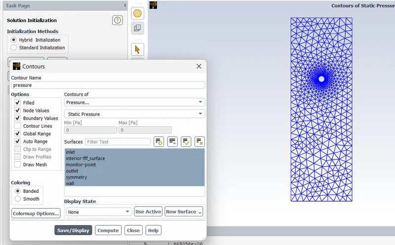
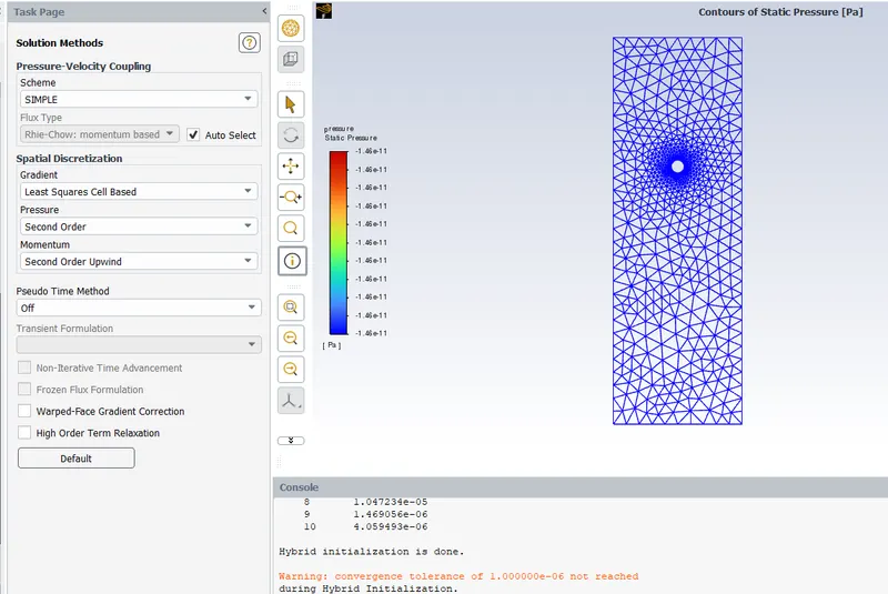
Initializing Domain - Hybrid
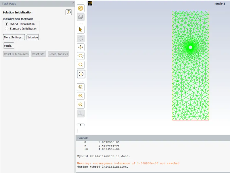
Creating Velocity Contours
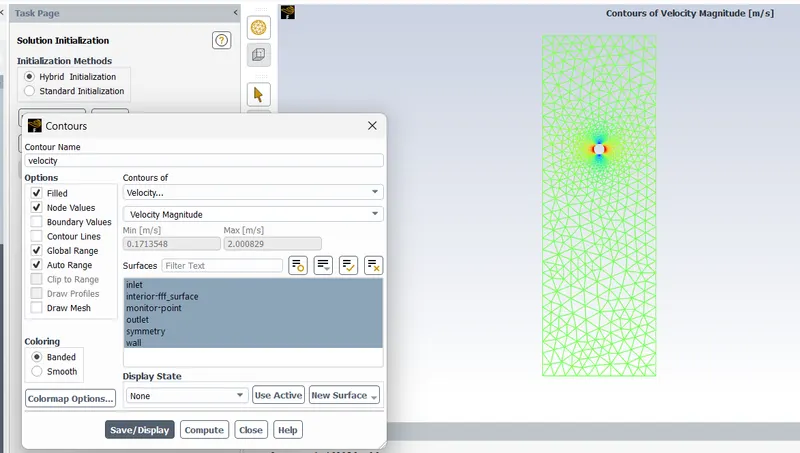
Initial Velocity Contours are shown
Pressure Contours
Solution Methods
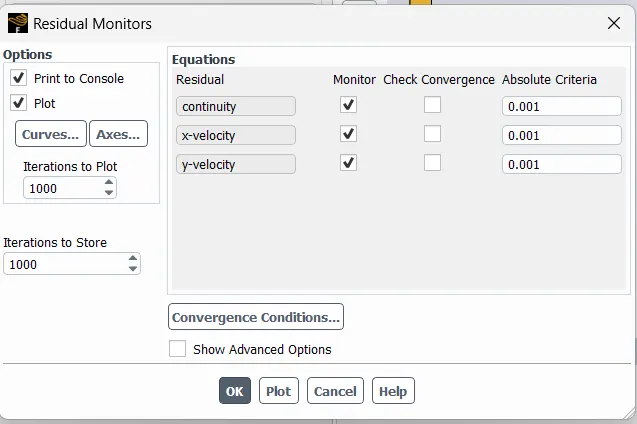
Residual Monitors
Unchecking Convergence Criteria
Reynold's Number (Re)
Re = U D / ν
free stream velocity = U
cylinder diameter = (D)">D
kinematic viscosity = v
Mesh Element Size changed to 0.2 m
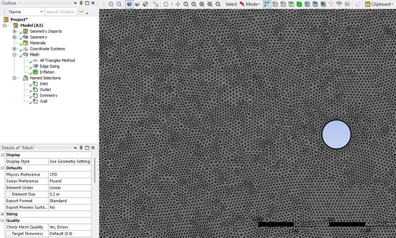
Vortex Shedding occurs when the Reynold's Number is greater than 40, even when the flow is laminar.
1. Simulating Flow with Steady Case
Re = 20
Mu = 0.1 m^2 / sec
Density = 1 kg/m^3
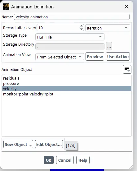
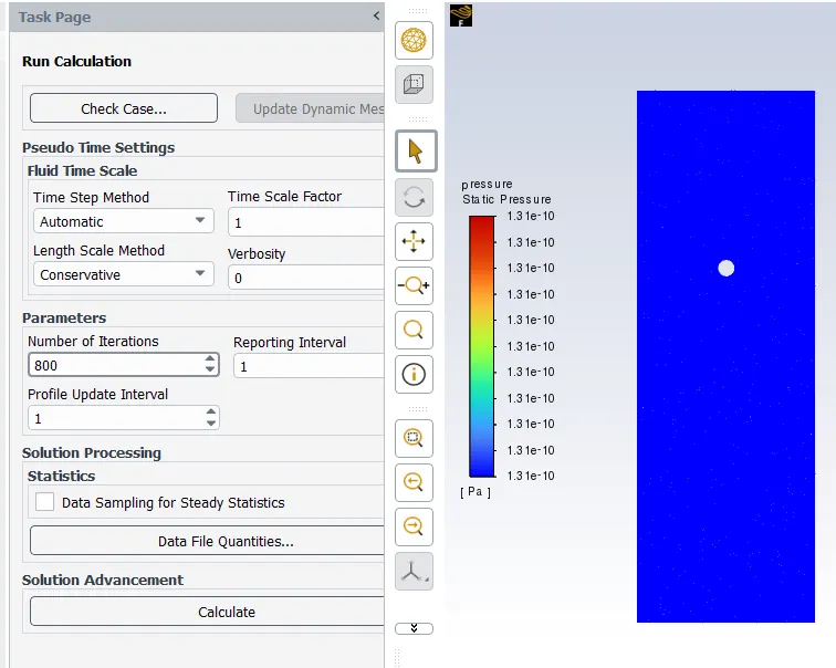
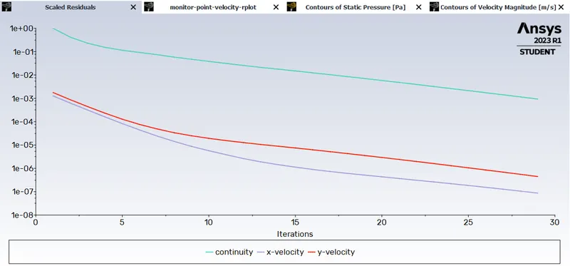
Solution is converged at 25th Iteration
Residuals
Vertex Average of Velocity Magnitude
Velocity Contour
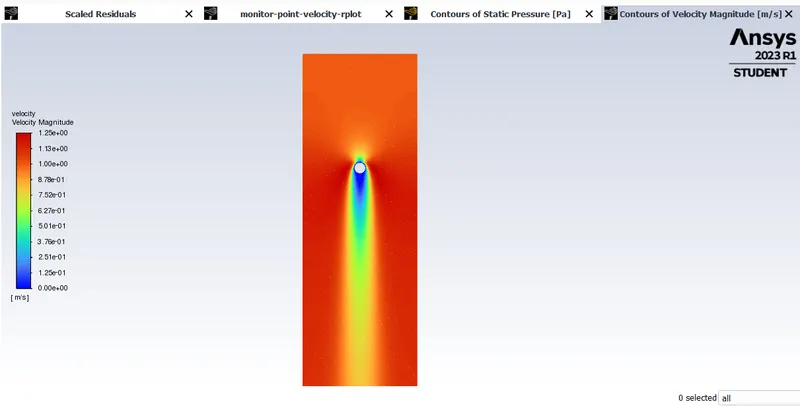
Pressure Contour
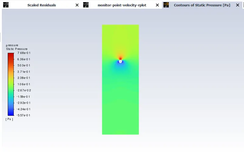
2. Simulating Flow with Unsteady Case
Re = 100
Mu = 0.02 m^2 / sec
Density = 1 kg/m^3
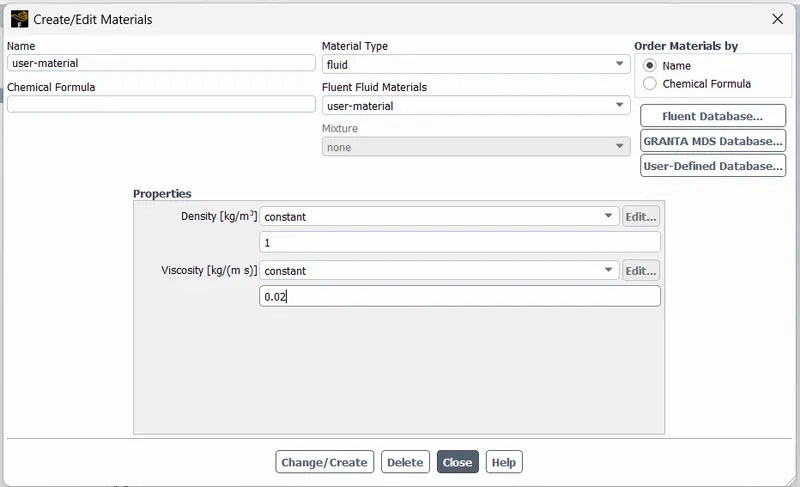
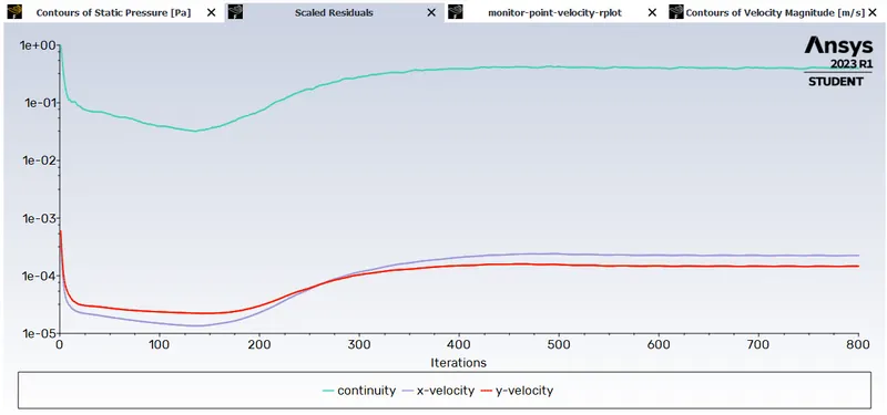
Residuals
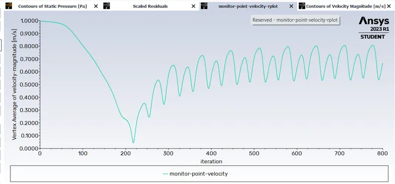
Vertex Average of Velocity Magnitude
Velocity Contour
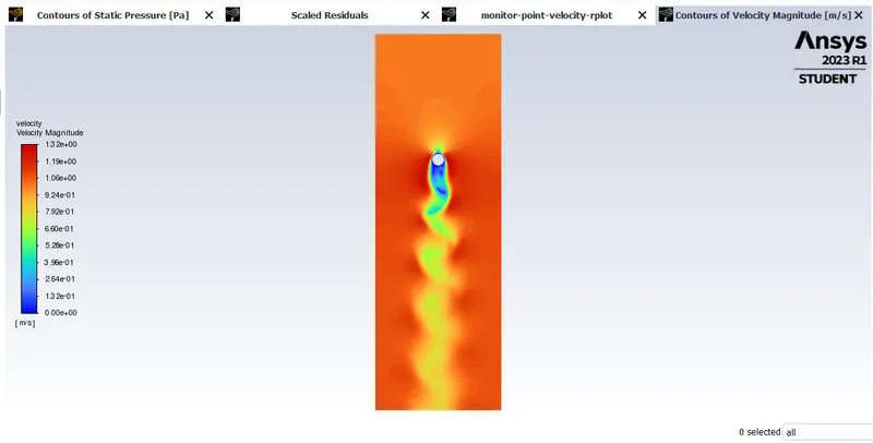
Pressure Contour
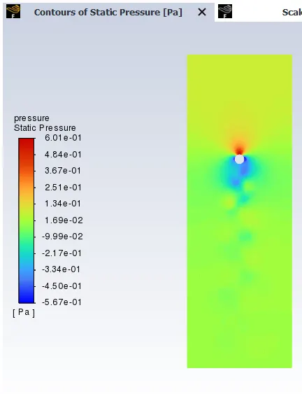
The Strouhal number is a dimensionless parameter describing the oscillating frequency of a flow.
The Strouhal Number is a function of the Reynold's Number.
Unsteady Case - Transient Simulation
Time Step Size = 0.03 sec
No. of Time Steps = 2000
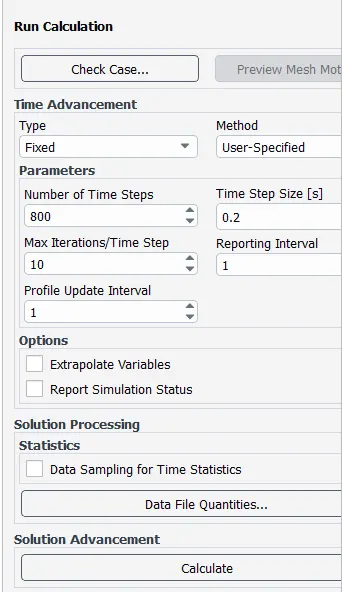
Scaled Residulas
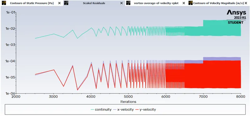
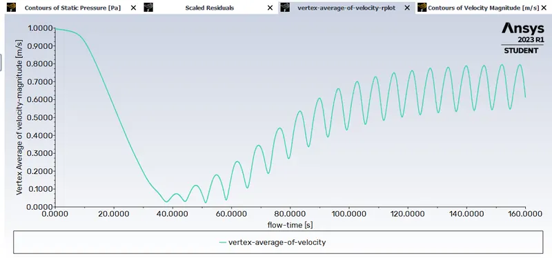
Vertex Average of Velocity at Monitor Point
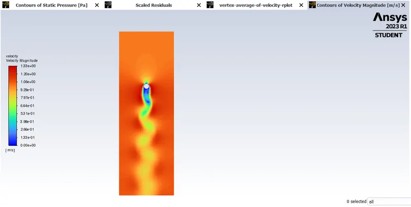
Velocity Contour
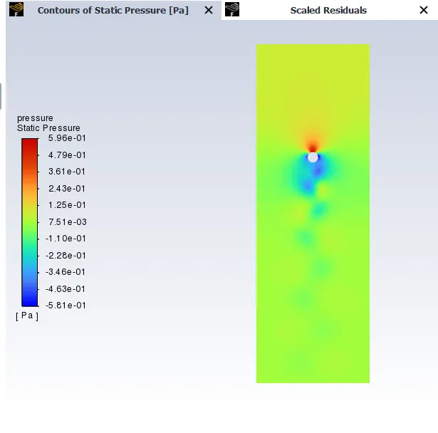
Pressure Contour
Strouhal Number = f * L / v
f = Frequency , No of Cycles / Time = 1 / (160 - 155.6) = 1 /4.4 = 0.22
L = Characteristic Length = 2 m
v = Flow Velocity = 1 m /sec
Strouhal Number = 0.22 * 2 / 1 = 0.44
Part - 2
- Calculate the coefficient of drag and lift over a cylinder by setting the Reynolds number to 10,100,1000,10000 & 100000. (Run with steady solver)
Formula for Reynold's Number :
Re = ρ * v * L / μ
Varying Velocity for Various Reynolds Numbers
ρ = 1 kg / m ^3
L= D = 2 m
μ = 0.02 kg / m - sec
Re = 100*v
| Re | Velocity |
| 10 | 0.1 |
| 100 | 1 |
| 1000 | 10 |
| 10000 | 100 |
| 100000 | 1000 |
Steady State Simulation
We need to calculate Coefficient of Lift and Drag.
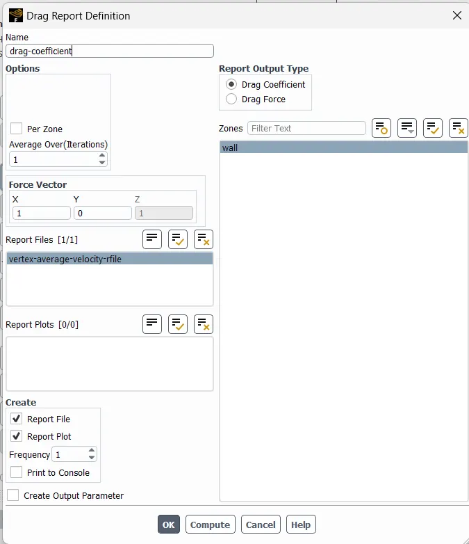
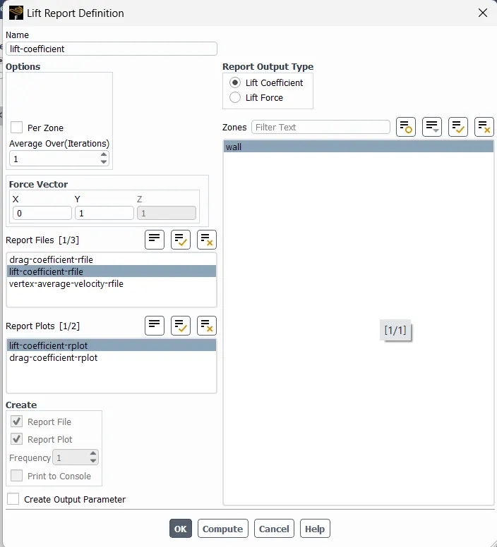
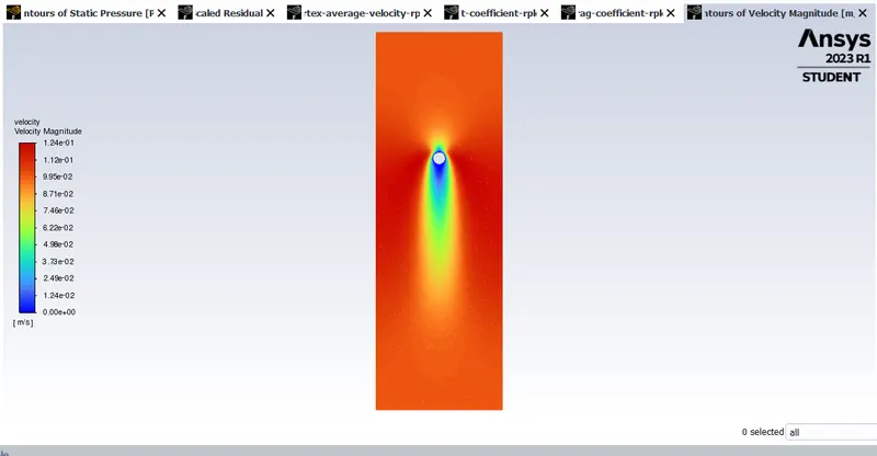
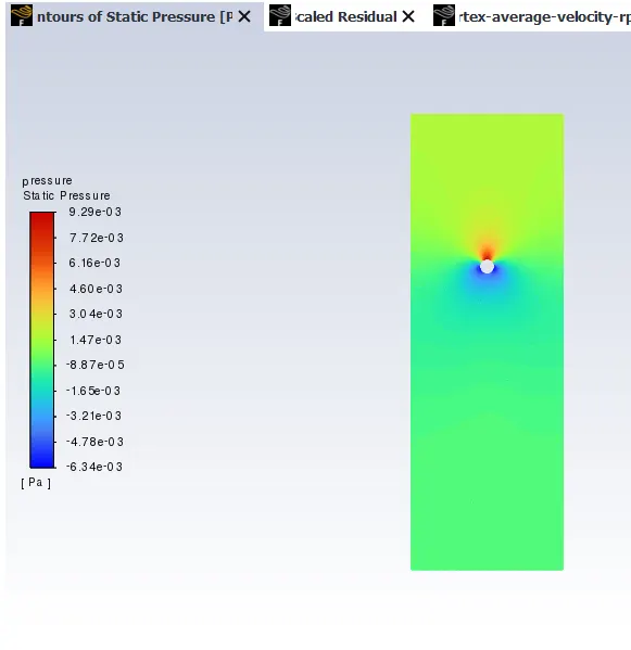
Case 1 - Reynold's Number = 10 , Velocity = 0.1
Project Schematic - B
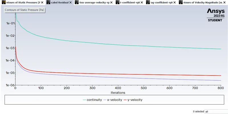
1. Scaled Residuals
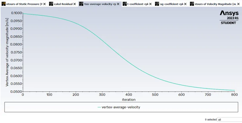
2. Vertex average of Velocity
3. Velocity Contour
4. Pressure Contour
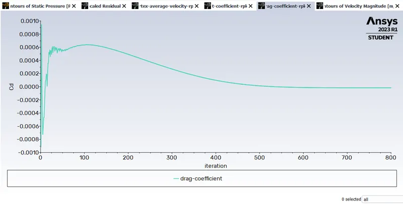
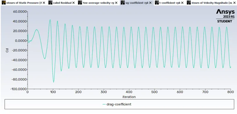
5. Drag Ceofficient
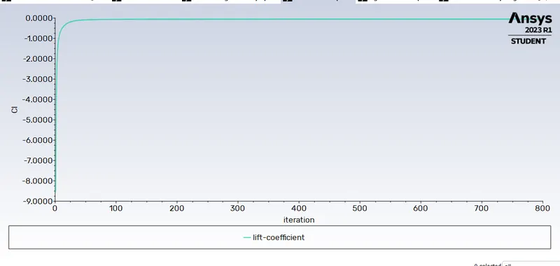
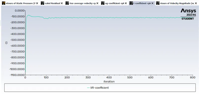
6. Lift Coefficient
drag-coefficient = -1.6031678e-05
lift-coefficient = -0.054394119
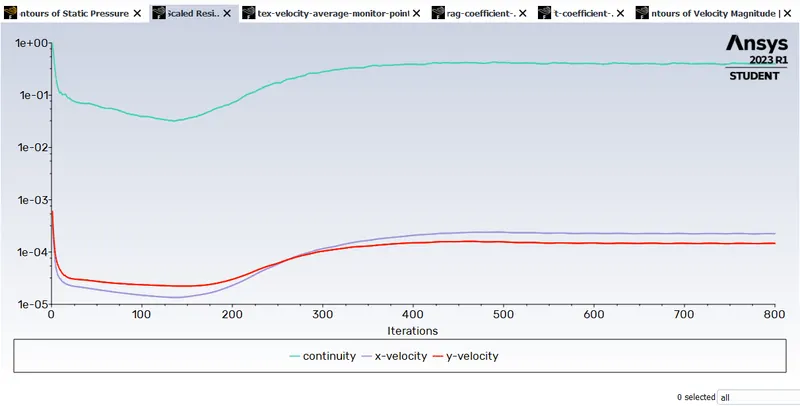
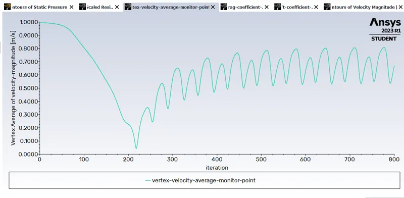
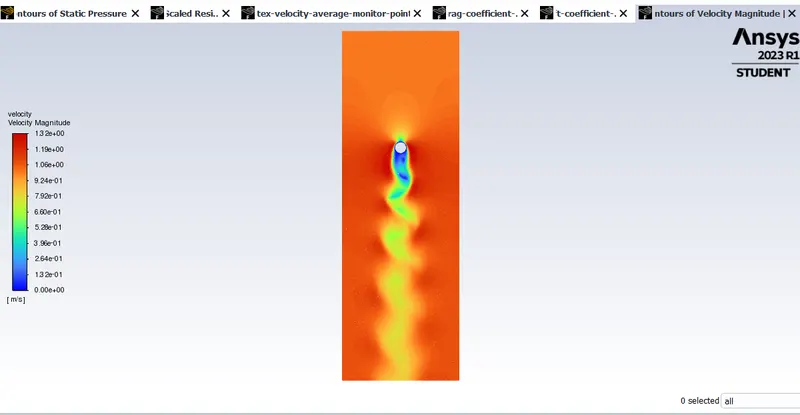
Case 2 - Reynold's Number = 100 , Velocity = 1
Project Schematic - C
1. Scaled Residuals
2. Vertex average of Velocity
3. Velocity Contour
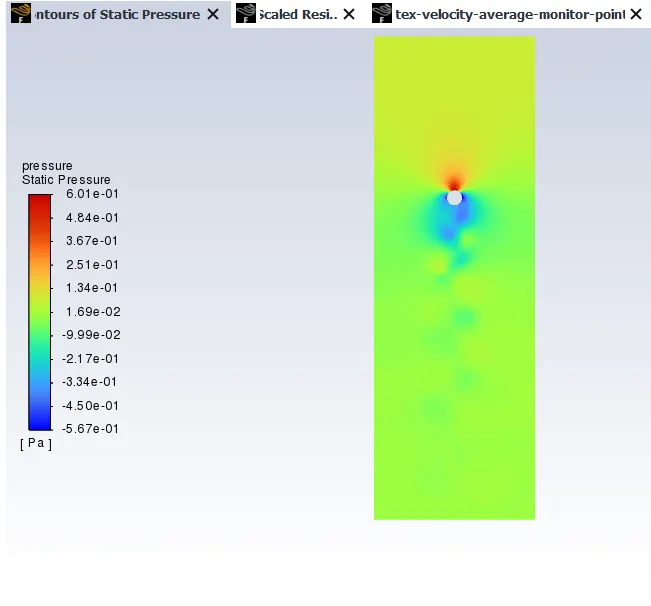
4. Pressure Contour
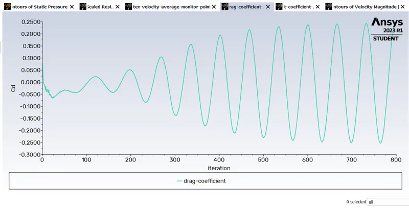
5. Drag Ceofficient
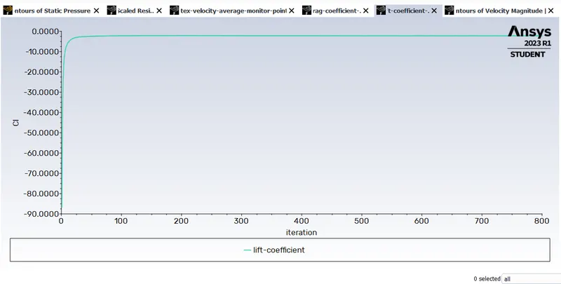
6. Lift Coefficient
drag-coefficient = 0.23951594
lift-coefficient = -2.2044919
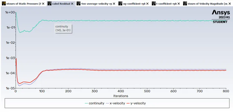
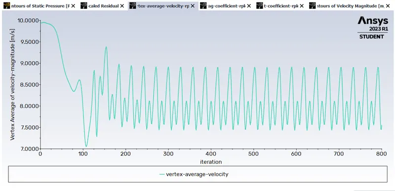
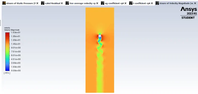
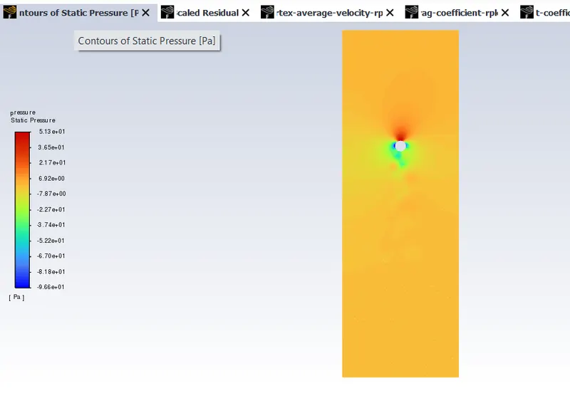
Case 3 - Reynold's Number = 1000 , Velocity = 10
Project Schematic - D
1. Scaled Residuals
2. Vertex average of Velocity
3. Velocity Contour
4. Pressure Contour
5. Drag Ceofficient
6. Lift Coefficient
drag-coefficient = -54.165498
lift-coefficient = -123.69882
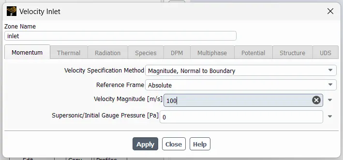
Case 4 - Reynold's Number = 10000 , Velocity = 100
Project Schematic - E
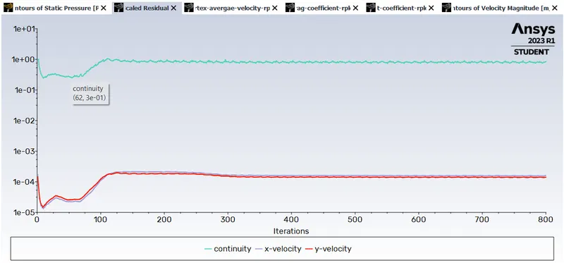
1. Scaled Residuals
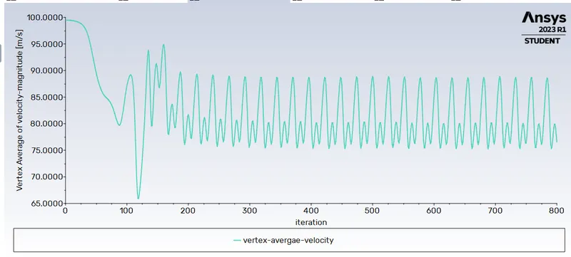
2. Vertex average of Velocity
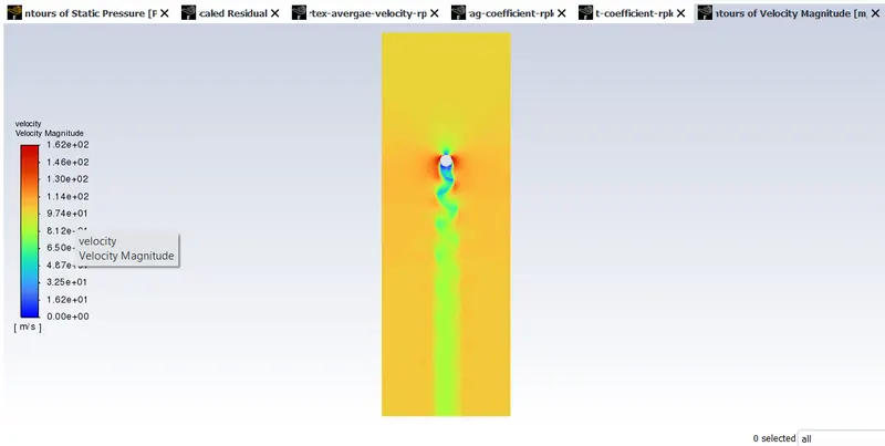
3. Velocity Contour
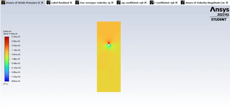
4. Pressure Contour
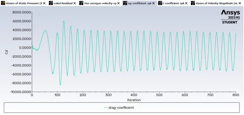
5. Drag Ceofficient
6. Lift Coefficient
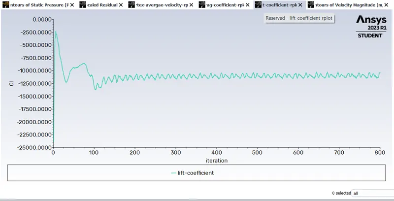
drag-coefficient = 3223.0228
lift-coefficient= -10398.516
Case 5 - Reynold's Number = 10000 , Velocity = 1000
Project Schematic - F
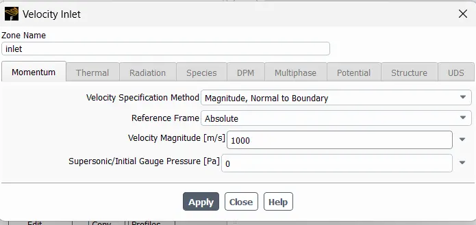
1. Scaled Residuals
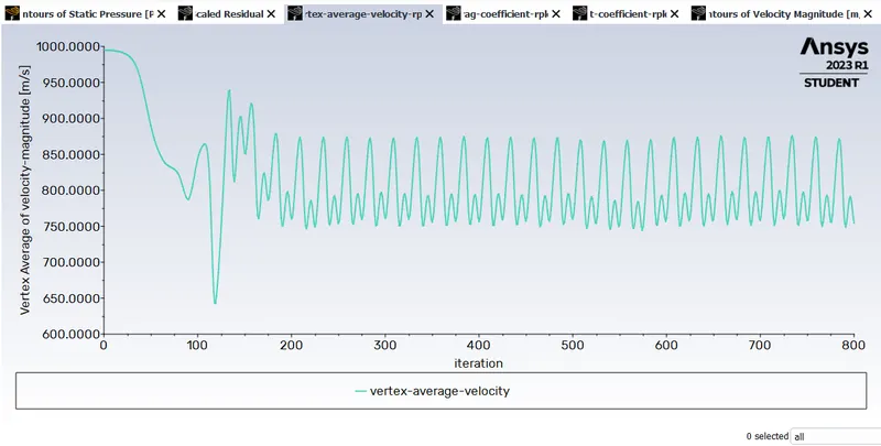
2. Vertex average of Velocity
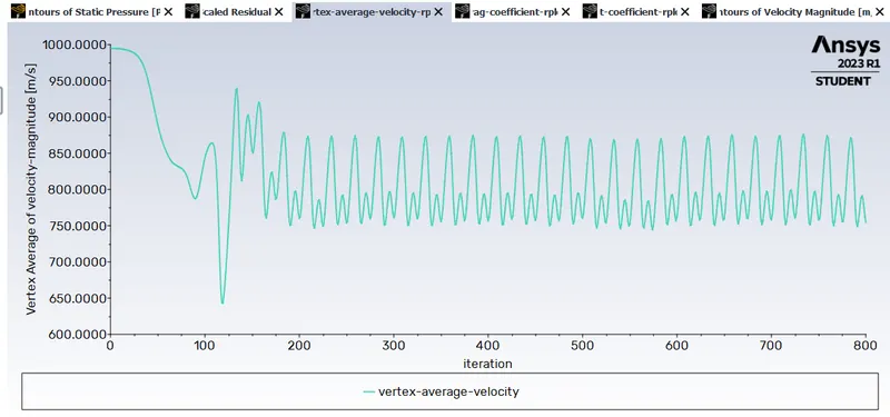
3. Velocity Contour
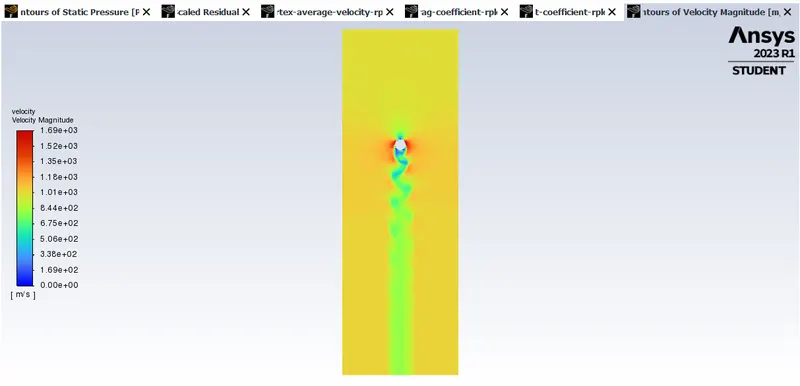
4. Pressure Contour
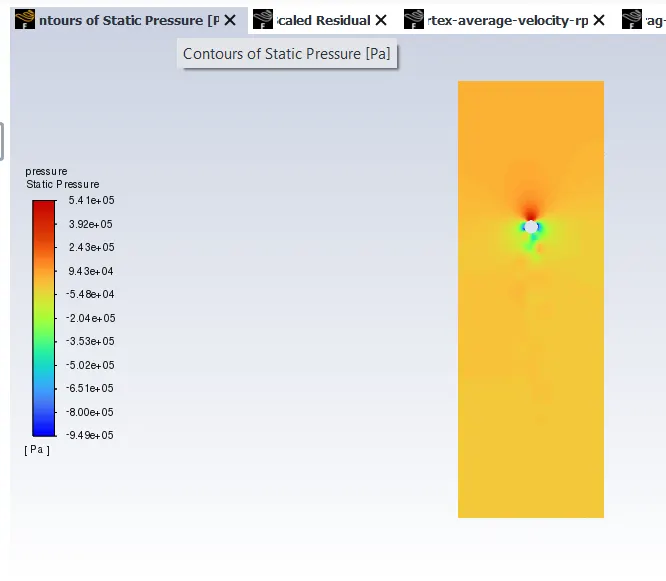
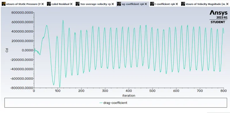
5. Drag Ceofficient
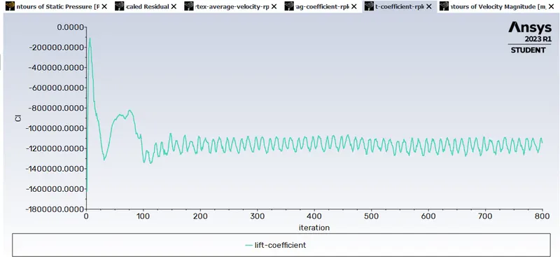
6. Lift Coefficient
drag-coefficient = 360110.23
lift-coefficient = -1150225
Conclusion -
1. Here the values of Cd and Cl are different than expected because of the different orientation of the geomerty.
Geometry is Vertical in this case.
2. If we look at the values of Cd and Cl, they tend to increase as the Reynolds Number is Increased.
3. Vertex Sheding phenomenon is captured more precisely in the case of Transient Simulation.