Week 5 - Rayleigh Taylor Instability

Introduction :-

Rayleigh Taylor instability:

From the Newtons law of viscosity, we know that even the fluid cannot resist the slightest shear force. Density is one of the main property of the fluid which the shear force can incorporate with it.

Depending upon the density we have lighter fluid like water etc and denser fluid like mercury, oil, honey etc.

Lord Rayleigh observed that when two liquids i.e lighter and heavier fluids are mixed together where the deser fluid is top on the lighter fluid, due to the gravity and the density variation the interface of the liquid is not stable. (i.e) water suspended on the oil .

So, the instability of the interface between the different densities of fluid when the lighter fluid is accelerated towards the heavier fluid is knowns as RAYLEIGH TAYLOR INSTABILITY.

Types of Instability and some practical CFD models that have been based on the mathematical analysis of Rayleigh Taylor waves:

Ritchmyer-Meshkov instability:

The Richtmyer-Meshkov instability arises when a shock wave interacts with an interface separating two different fluids. It combines compressible phenomena, such as shock interaction and refraction, with hydrodynamic instability, including nonlinear growth and subsequent transition to turbulence, across a wide range of Mach numbers.

Plateau–Rayleigh instability:

The Plateau–Rayleigh instability, often just called the Rayleigh instability, explains why and how a falling stream of fluid breaks up into smaller packets with the same volume but less surface area. This fluid instability is exploited in the design of a particular type of ink jet technology whereby a jet of liquid is perturbed into a steady stream of droplets.

Kelvin–Helmholtz instability:

can occur when there is velocity shear in a single continuos fluid, or where there is a velocity difference across the interface between two fluids. An example is a wind blowing over water: The instability manifests in waves on the water surface. More generally, clouds, the ocean, Saturn's bands, and the sun's corona show this instability.

Practical CFD models:

SPH method(Smoother particle hydrodynaics)

Smoothed-particle hydrodynamics (SPH) is a computational method used for simulating the mechanics of continuum media, such as solid mechanics and fluid flows.Smoothed-particle hydrodynamics is being increasingly used to model fluid motion as well. This is due to several benefits over traditional grid-based techniques. First, SPH guarantees conservation of mass without extra computation since the particles themselves represent mass. Second, SPH computes pressure from weighted contributions of neighboring particles rather than by solving linear systems of equations. Finally, unlike grid-based techniques, which must track fluid boundaries, SPH creates a free surface for two-phase interacting fluids directly since the particles represent the denser fluid and empty space represents the lighter fluid.

SINGLE-FLUID MODEL

A typical approach used for the analysis of two-phase flows is a mixture model, i.e. the individual fluid phases are assumed to behave as a flowing mixture described in terms of the mixture properties. The applied single-fluid model is a five-equation model consisting of the mass, momentum and energy equations for a vapor/liquid mixture, and two equations describing the formation and growth of the liquid phase.

TWO-FLUID MODEL

In the two-fluid model, separate sets of the governing equation for the vapor and liquid phases have been used. The interaction between the droplets and the heat exchange between the liquid phase and the solid boundary are not modelled here as well. Additionally, the velocity slip between vapor and the liquid phase is in this model taken into account.

Turbulence model

Turbulence models are needed to predict the average mixing behaviour in flows that are on average one- or two-dimensional. The approach to the construction of tile turbulence model is guided by the experimental behaviour.The equations governing turbulent flows can only be solved directly for simple cases of flow. For most real life turbulent flows, CFD simulation use turbulent models to predict the evolution of turbulence. These turbulence models are simplified constitutive equations that predict the statistical evolution of turbulent flows.

Aim :-Perform the Rayleigh Taylor instability simulation for 2 different mesh sizes with the base mesh being 0.5 mm.

Procedure :-

• Open spaceclaim.
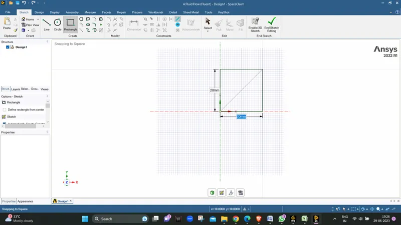
• Make a rectangle of 20 mm X 20 mm from origion using recgangle tool
• 
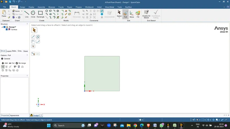
• Now we will use pull command to convert the rectangle to surface.
• 
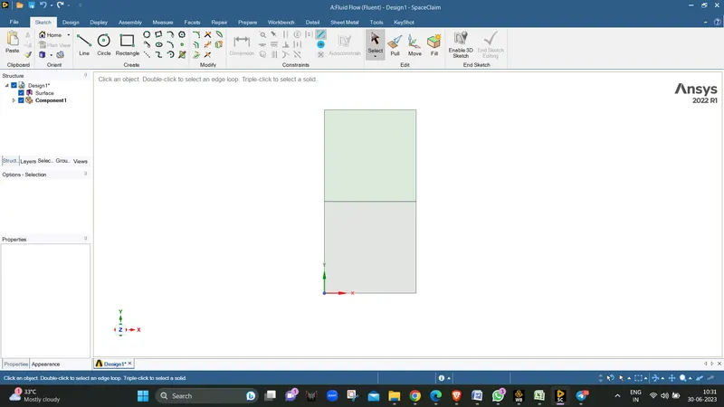
• Then we will create a new component ans create another surface of same size on top of the previous surface.
• 
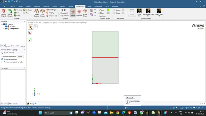
• Then we will use share tool to share the interface between both the surfaces.
• 
• 
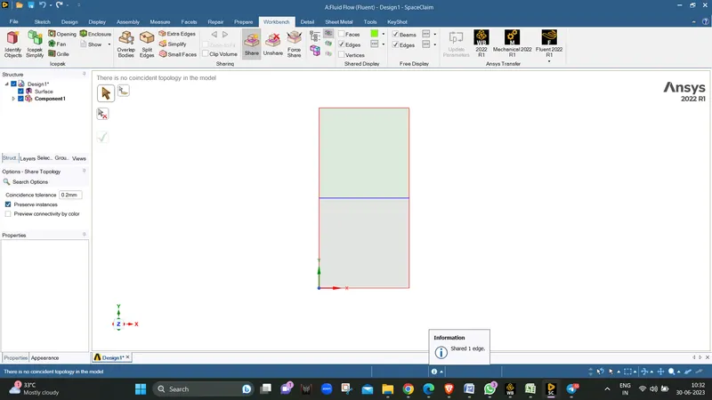
• Next we will go for meshing and we will perform mesh independent study to perfrom atleast 3 simulations by varying the element sixe in mesh.

MESHING :-

• we will first go with 0.5 mesh and when meshing will be done we will move to setup
• 
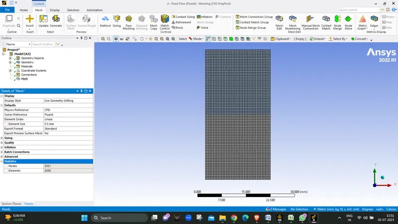
• Now we can see the number of elements are 3200 with mesh size as 0.5 mm
• Now we will lead to the setup part .

SETUP :-

• We will use Transient state solver , in muliphase we will use VOF (Volume Of Fluid) model and our viscous model will be laminar (we can run this with k omega sst but we are not using it here as there is no application of external force n fluid) we will be enabling gravity whose standard value we have as 9.81 m/s in downward direction.
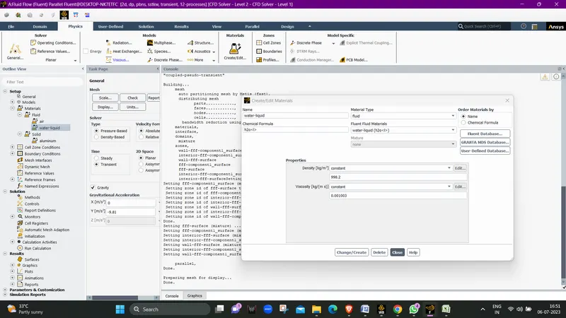
• We will be assigning 2 different materials one is air and other is water in which primary phase will be air and secondary phase will be water.
• We won't be using any energy equation and will be using default coupled solver and will be patching the surfaces.
• Opening setup we will enable Transient and Gravity.
• 
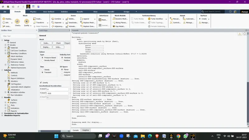
• We will change viscous to laminar model
• Now we will add material properties of air and water.
• 
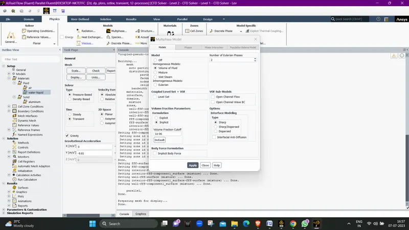
• Now we will select the multiphase model.
• We will select volume of fluid and implicit formulation and click apply.
• 
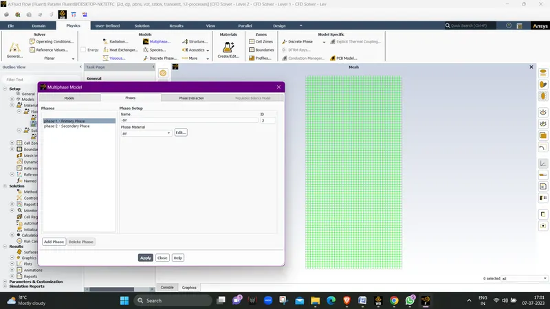
• Now we go in the hases menu in the same dialogue box.
• We will select primary phase as air and rename phase 1 to air.
• 
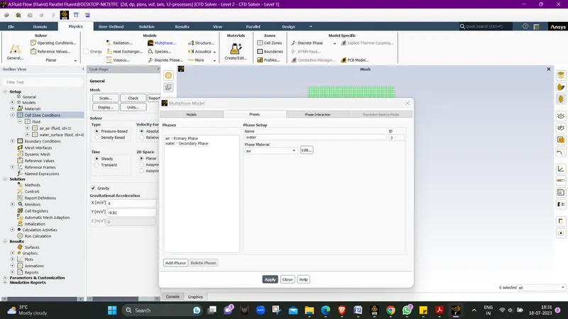
• We will select secondary phase as water and rename phase 2 to water and click apply and close the wndow.
• 
• We will now go to solution tab and initialize the simulation and we will create a contour plot of phases and select phase 1 in the phase column and click ok lets see what happen.
• 
• 
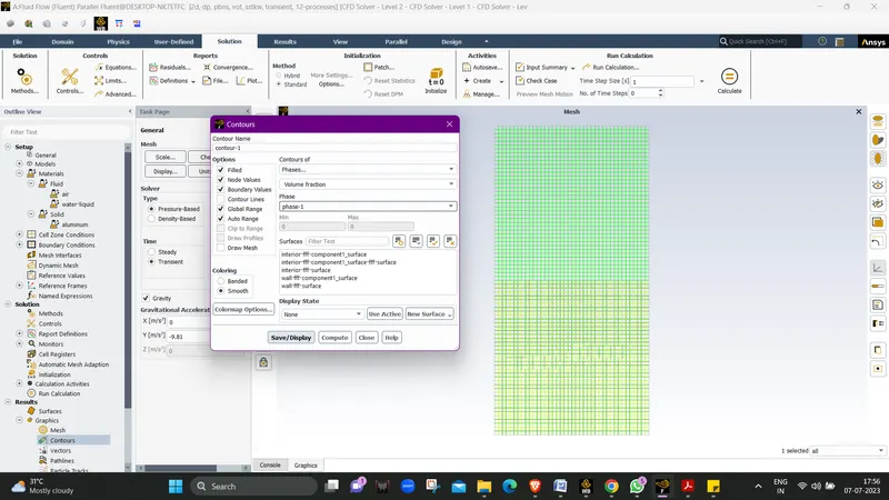
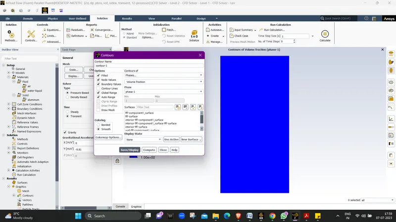
• we can see only 1 phase which is liquid but we are performing the simulation for water and air interaction so we need to have water as phase 2 so for that we have to patch the surfaces.
• 
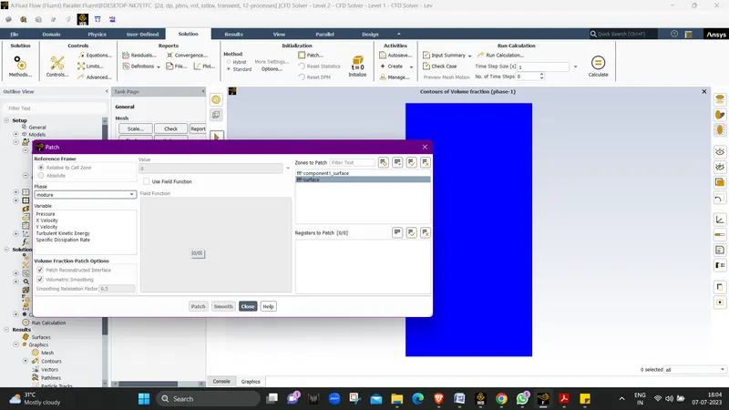
• We will click on patch and patch the two surfaces as if we donot patch the liquids we won't be able to see the simulation results. so we will patch water with volume fraction of 1 and air with volume fraction of 0, and we will right click on contour 1 and select update.
• 
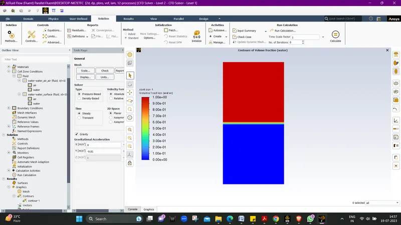
• Now we will create anmation we will click on create in solution tab under activities and select solution animation.
• 
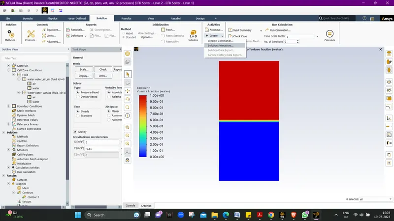
• As we open Solution Animation we will select contour-1 and click on Use Active and let the name be Animation-1. Use Active will take the current contour ase its initial frame.
• 
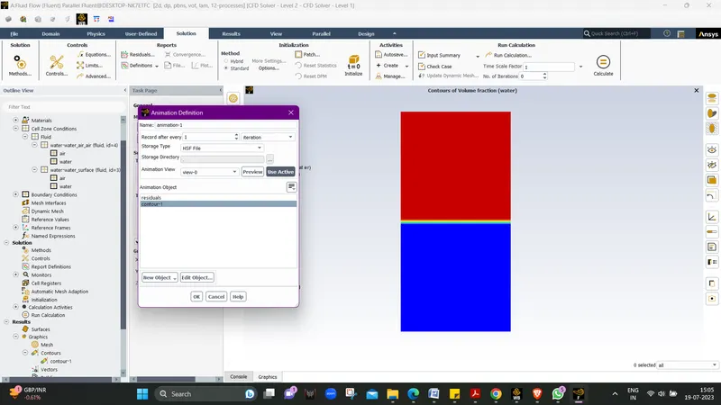
• NOw we will select the time step size
• If we have smaller time step the computational time will be more but it will give good results
• if we use bigger time step the computational time will be more but it will give void exception error which means due to higher time step size it won't be able to capture fluid motion in every element.
• And it also depends on the mesh if acording to mesh size we are selecting higher time stepit will show the void exception error.
• like if we are having a mesh of 0.1 mm and we are using the time step size as 0.01s then it will create a void exception error so we won't get the solution.
• Although deciding time step size is hit and trial method but we shouls start with the smaller time steps and can also increase the time step size gradually using a script which can be written in matlab and then added to the simulation
• we can do this by giving first 500 time steps with smaller time step and then incrrease the time step size for next 500 time steps which will decrease the computational time. lik this we can gradually increse time step size.
• simulation time is product of the time step and number of steps
• Simulation Time = Time step x Number of steps.

For the first case we can calculate the simulation time

Simulation Time = 0.01 x 200 = 2 sec

this is just an assumption we can run for further number of steps if the simulation is not done to the extent we want it to happen.

• Now for this case we have mesh of 0.5 mm and we will use time step of 0.01 s and run the simulation.
• We run the simulation for 2000 time steps
• 
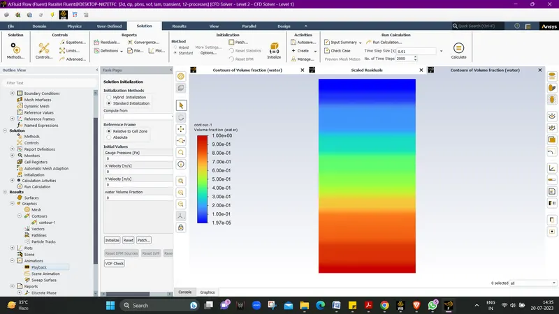
• Now we will run the second case with a more finner mesh with 0.1 mm element size.
• we will use timestep of 0.001s and use number of time steps as 4000 we can see in the screen tht heavier fluid have taken place at bottom.
• 
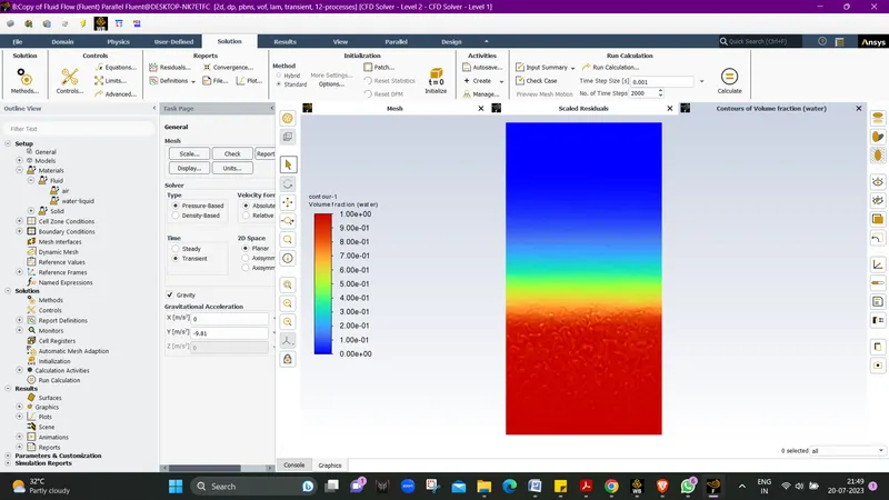
• Now we will run one more simulation with water and user-defined material (density = 400 kg/m³, viscosity = 0.001 kg/m-s) for refined mesh.
• Now we will compare the results for the simulation for all the cases

Results :-ol

Cases	Solution Animation
Case 1
Case 2
Case 3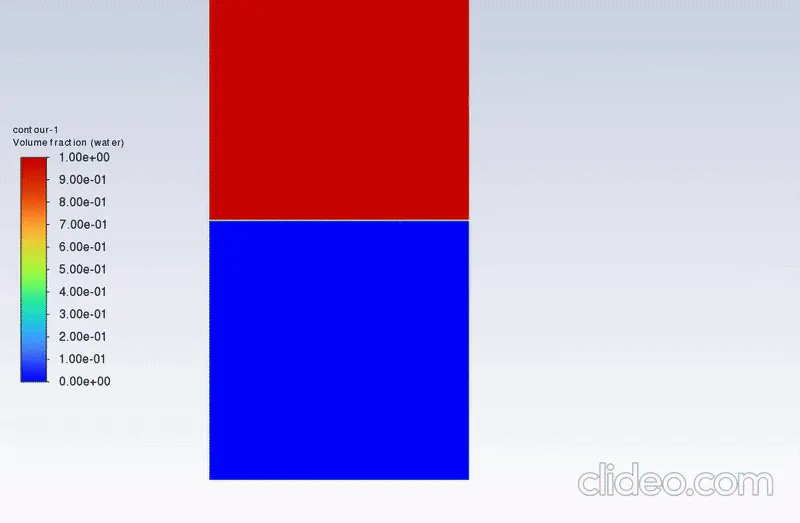

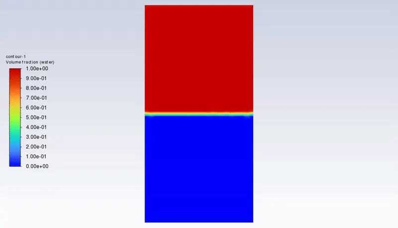
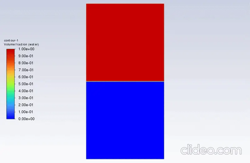
From the above animations we can see that in case 1 we have greater mesh size due to which the the fluid mixed in form of layers as compared to case 2 where the fluid mixed in the form of particles and which shows us clearly how denser fluid takes place of a less denser fluid due to gravity .

Talkinf about the case 2 and case 3 we can see that the in case 3 the denser fluid which ids ater taking more time to settle down as compared to case 2 and the mesh size for both the cases is same. this happened due to density difference between the fluids in case the density difference was bigger and in case 3 density difference was small.

from the experiment we can se that the time taken is more when the density difference between the two fluid is less as we know the denser fluid take place of less denser fluid but when difference is less the resistance to deform is more due to which it takes more time dor denser fluid to take place of a less denser medium.

Atwood number (A)

The Atwood number (A) is a dimentionless number in Fluid Dynamics used in the study of Hydrodynamic Instablities in density stratified flows. It is a dimensionless density ratio defined as

A = (ρ₁ − ρ₂)/(ρ₁ + ρ₂)

where

ρ₁ = Density of heavier fluid

ρ₂ = Density of lighter fluid

Density of heavier fluid (water) = 998.2 kg/m³

Density of Air = 1.225 kg/m³

^{Density of User-defined fluid = 400 kg/m3}

Atwood number for case 2 :- (998.2 - 1.225 )/(998.2 + 1.225 )

= 996.975 / 999.425

= 0.99754

Atwood number for case 3 :- (998.2 - 400 )/(998.2 + 400)

= 598.2 / 1398.2

= 0.42783

Therefore A_case2 > A_case3

We can see that the Atwood number for Case 2 is more then case 3. So higher the atwood number the time taken for denser fluid to take place of low denser fluid is less.