Week 5 - Rayleigh Taylor Instability

AIM: To perform the Rayleigh Taylor instability simulation for 2 different mesh sizes with the base mesh being 0.5 mm. Compare the results.

THEORY:

Rayleigh–Taylor instability:

The Rayleigh–Taylor instability, or RT instability is an instability of an interface between two fluids of different densities which occurs when the lighter fluid is pushing the heavier fluid.

Practical CFD models that have been based on mathematical analysis of RT waves

• Kelvin-Helmholtz instability:

This theory states that, this instability typically occurs when there is velocity shear in a single continuous fluid, or additionally where there is a velocity difference across the interface between two fluids. A common example is seen when wind blows across a water surface, the instability constant is able to manifest itself through waves on water surface.

• Richtmyer–Meshkov instability:

This theory states that, this type of instability occurs when there is an impulsive accelaration between two fluids. This type of instability can occur when there is a shock at greater speeds. The development of the instability begins with small amplitude perturbations which initially grow linearly with time.

• Plateau-Rayleigh instability

The Plateau–Rayleigh instability, often just called the Rayleigh instability, explains why and how a falling stream of fluid breaks up into smaller packets with the same volume but less surface area. It is related to the Ryleigh- taylor instability. and is part of a greater branch of fluid dynamics concerned with fluid thread breakup.

Atwood Number:

The Atwood number (A) is a dimensionless number in fluid dynamics used in the study of hydrodynamic instabilities in density stratified flows. It is a dimensionless density ratio defined as

where

ρ₁= density of heavier fluid

ρ₂= density of lighter fluid

For A close to 0, RT instability flows take the form of symmetric "fingers" of fluid; for A close to 1, the much lighter fluid "below" the heavier fluid takes the form of larger bubble-like plumes.

PROCEDURE:

• Open the Ansys Spaceclaim and draw two squares of dimensions 20x20 mm and use pull tool to make it plane surface. The upper sqaure of the geometry represents water and lower square represents air, as shown in figure.
  
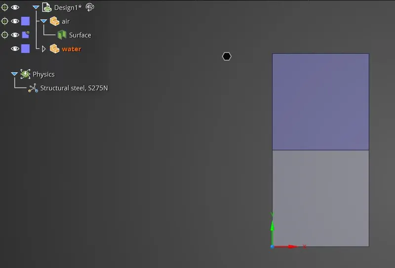
• Share the topological data between the two geometries by unabling the share tool.

CASE 1:

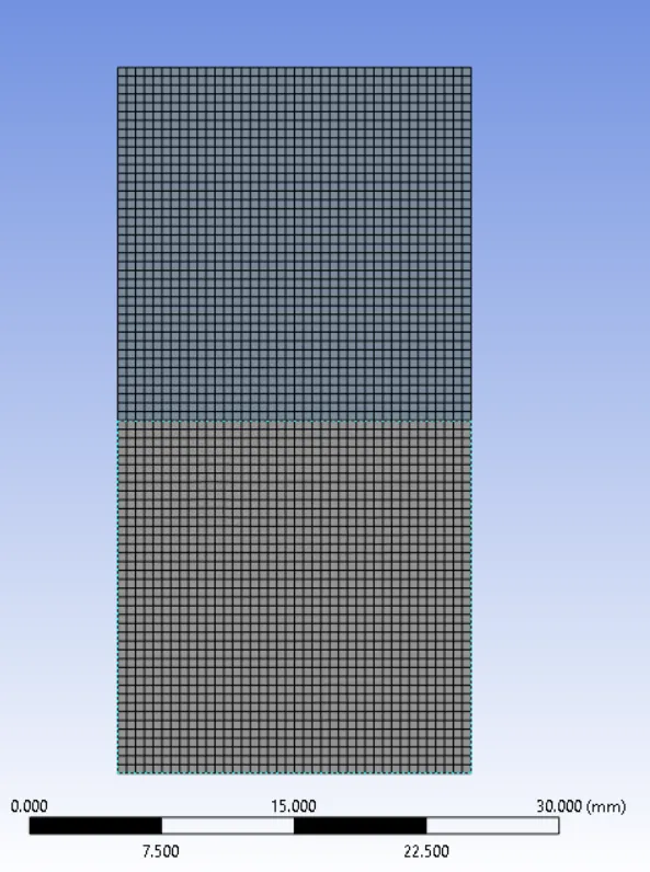
• Then the geometry is meshed with an element size of 0.5mm and consider it as a baseline mesh
• And number of elements generated are 3200 and number of nodes are 3321 and the generated mesh is shown below.
  
• Then name the geometries as air and water, after that move to the solvent setup part.
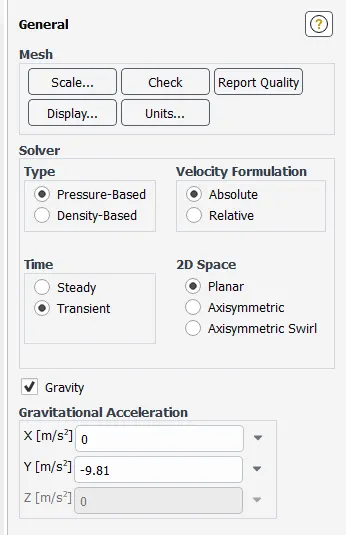
• Here, select the transient state flow, and select the Gravity and give the gravity value as -9.81 in the y coordinator section.
  
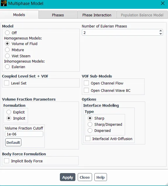
• After, that give the laminar case in the viscous model, and goto multiphase model select volume of Fluid and here the 2 Eulerian phases are air and water.
  
• And Intialize the t = 0, after that patch the volume of fluid od air as 0 and volume of fluid of water as 1. After that create a vaolume fraction conture to the all surface of the model, And also, create surface aimation on the focused contour then set the run time set up to 0.05 and run 1500 iterations and observe the results.
  
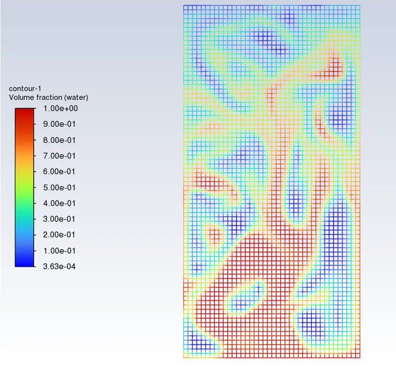
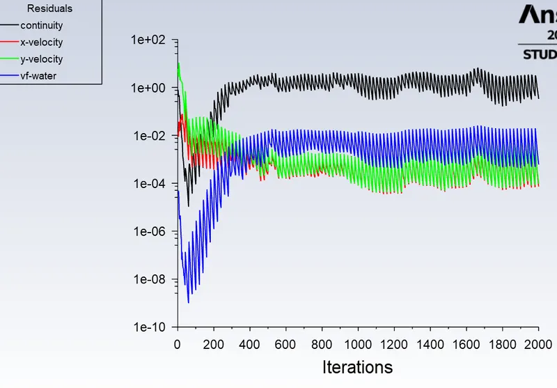
• Atwood number value of this case is calculated as below:
  
  

  ρ₁= density of water = 998.2 kg/m^3

  ρ₂= density of air = 1.225 kg/m^3

  A = (998.2 - 1.225)/(998.5 + 1.225) = 0.9972

  
  CASE 2:
• In the case 2 refine the mesh with element size 0.25mm and generate mesh. Here, the Number of Elements generated are 12800 and the number of Nodes count are 13041.
  
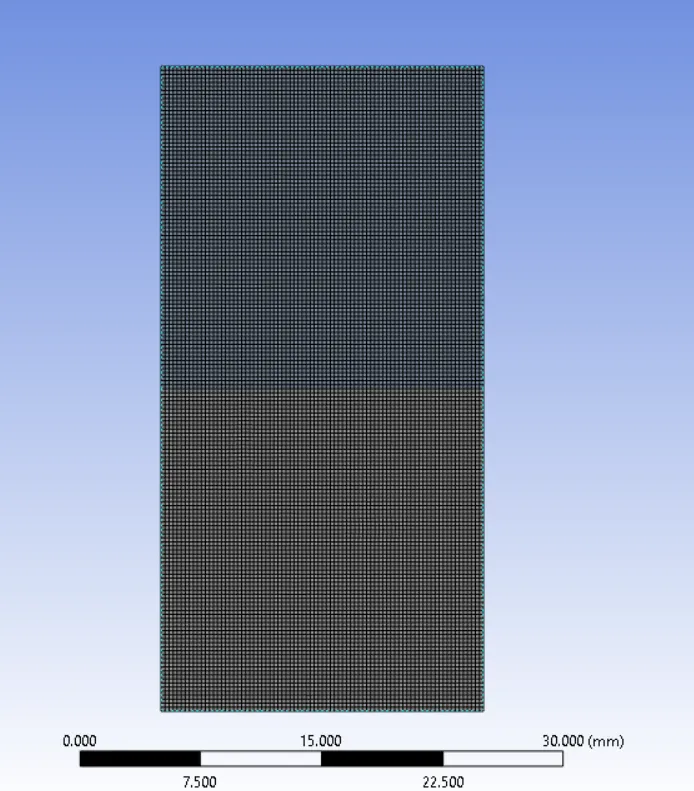
• And run the same setup to the above meshed geometry and the results are mentioned below.
  
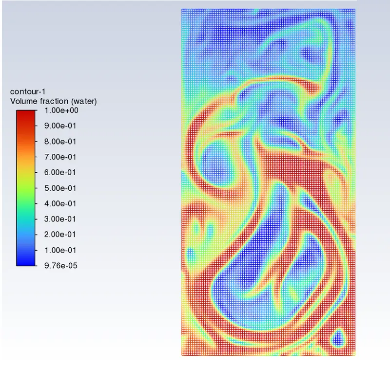
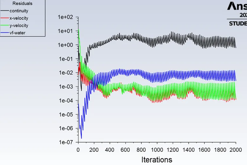
• Atwood number value of this case is calculated as below:
  
  

  ρ₁= density of water = 998.2 kg/m^3

  ρ₂= density of air = 1.225 kg/m^3

  A = (998.2 - 1.225)/(998.5 + 1.225) = 0.9972

CASE 3: Here, mesh the geometry with element size of 0.3mm, After meshing there are 8978 elements number and 9180 nodes are generated.

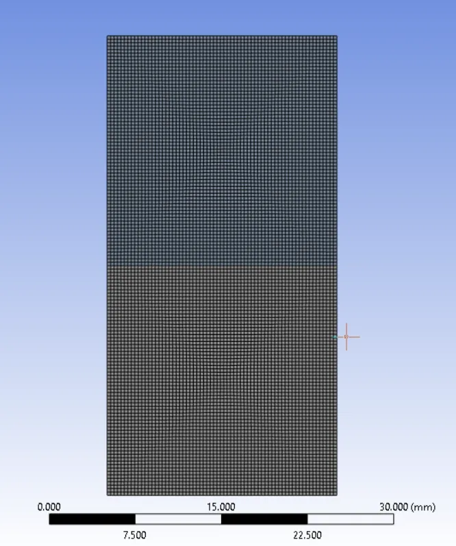
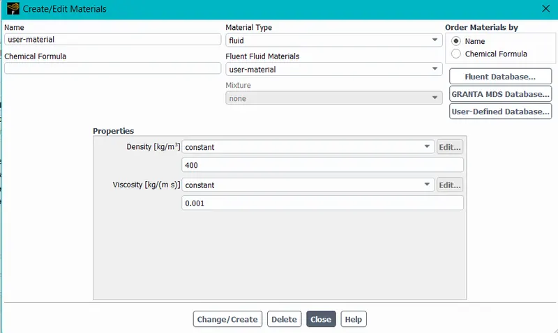
• Then move to setup part, and take an user defined material of density = 400 kg/m³, viscosity = 0.001 kg/m-s.
  
• Then run the setup and observe the generated results.
  
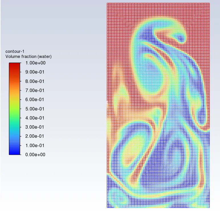
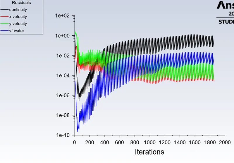
• Atwood number value of this case is calculated as below:
  
  

  ρ₁= density of water = 998.2 kg/m^3

  ρ₂= density of air = 400 kg/m^3

  A = (998.2 - 400)/(998.5 + 400) = 0.4277

CONCLUSION:

Case number	Mesh Element size	Number of Elements	Atwood value
CASE 1	0.5	3200	0.9972
CASE 2	0.25	12800	0.9972
CASE 3	0.3	8978	0.4277

Here Finally we Stimulated there diffent mess models in the ANSYS FLUENT under the Academic licence limits and the results are mentioned above, Here we observe that finer mesh captures the instability better than the coarse mesh, and we run the the model for every time step of 0.005sec, due to this the computational time is long and the results are captured accurately. And also, for the Atwood number close to 0, RT instability flows take the form of symmetric fingers of fluid, and also when Atwood number close to 1, the much lighter fluid below the heavier fluid takes the form of larger bubble-like plumes.

The Animated results are attached in this following link. https://drive.google.com/drive/folders/1nuDDhT8cXfXq7-Cgv9vlt7Hr6AkKsFcN?usp=sharing