Week 5 - Rayleigh Taylor Instability

Introduction:

Rayleigh Taylor Instability is the phenomenon first observed by Lord Rayleigh and G.I. Taylor. In this phenomenon lighter liquid is supported by the heavier liquid and when there is disturbances at the interfaces the heavier liquid pushes the lighter liquid also the lighter liquid due to its low density pushes tries to come up and in turn pushes the heavier liquid. Due to this phenomenon flow instabilities arises; this is nothing but Rayleigh Taylor Instability. This phenomenon is observed in many practical applications, such as in die casting. When hot liquid metal is poured into the cavity, the cavity is present with some air, due to this the higher density hot liquid metal pushes the sir inside the cavity and air in turn pushes the liquid and hence there are instabilities, due to this there can be manufacturing defects. Also, in combustion chamber of air breathing or rocket engines when atomized fuel is injected into the combustion chamber, to increase the process of mixing and combustion this phenomenon is used.

Practical examples:

It is utilized for non-equilibrium reactive flows that are premixed, partially premixed, or not at all. It can handle chemical reaction- and external force-driven subsonic and supersonic flows. It was created to look at non-equilibrium hydrodynamic and thermodynamic effects in phase separation processes. It calculates the departure amplitude from thermodynamic equilibrium based on the characteristics of thermodynamic non-equilibrium.

Procedure:

1. Create geometry in Spaceclaim. In the model tree create 2 different component for air and water phase both. Make sure that at the end share topology is ON.
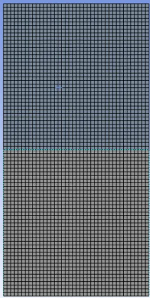
2. As the geometry is regular and structured, the mesh is structured, for different cases, the mesh size is changed accordingly.
3. Open the fluent and select the transient model, check the gravity option and give value for g=-9.81 in y direction, as the geometry is made in XY plane.
4. The case is setup and laminar model is selected. At first extra phase is added i.e water; from fluent database. Then select the Multiphase model and select the Volume of Fluid Method. In VOF method select the implicit method as explicit method will pose restrictions on CFL number and the solution might not converge.
5. Go to the solution and initialize the problem. After initialization each cell should be assigned in which phase, they are present. This is ensured by patching.
6. After this, to see how the phase mixing occurs. a contour is selected, and animation is created.
7. Input the number of time steps and time step size and hit run button.

What is Atwood number and what is its significance

The Atwood number measures the difference in density between two fluids or gases. It tells us how much heavier one fluid is compared to the other.

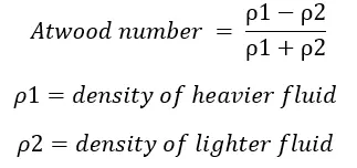
If the Atwood number is high, then it means there is significant difference between density and due to this there will be strong force in mixing. Due to this heavier fluid will sink in the lighter fluid with more force. This means that Rayleigh Taylor Instability will be high and intermixing between two phase will be chaotic and turbulent

So, if Atwood number is low then the mixing strength will be low and Rayleigh Taylor Instability will be low, hence lower mixing force.

Atwood Number gives the physical significance of how the heavier and lighter liquid interacts while mixing. Now to capture this the domain of interest needs to be discretized.

There are two different cases ,case A with base mesh size of 0.5mm and case B with mesh size of 0.15mm. Also in Case C the material is changed and the effect of change in Atwood number for same mesh size as of Case B is observed.

CASE A: Mesh size = 0.5mm

Geometry:

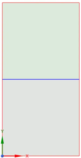
Mesh: Number of elements:3200 and Number of Nodes:3321

CASE B: Mesh size = 0.15mm

Mesh: Number of elements:47432 and Number of Nodes:47895

CASE C: r=400 kg/m3 and m=0.001 kg/ms and Mesh size is 0.15mm.

Same mesh size as of Case B is used.

Solution aniimation

https://drive.google.com/drive/folders/1vPapOFxAt8XfgsZEMSz6Tjcqut9H0UMi?usp=share_link

Results and Discussion:

As the Atwood Number for Case A is high , we can see that the intermixing of both phases is very chaotic and turbulent. This is because of high density differences between water and air. Also it can be observed that the motion is not captured in a better way due to coarser mesh. So for same Atwood number the mesh size is made more finer and it can be seen that the mixing is better observed. Due to finer mesh size the computation time is also increased.

Now for lower Atwood Number for same mesh size as of Case B, it can be observed that the mixing intensity or Instabilities are very low as compared to Case B. This is due to lower density difference between two phase or fluids.

Transient analysis is used in Rayleigh-Taylor instability simulations because instability itself is a transient phenomenon.

In a steady-state simulation, the system is assumed to reach a stable equilibrium where the fluid interface between the two fluids remains fixed and does not evolve with time. However, the Rayleigh-Taylor instability involves the dynamic growth and evolution of the interfacial structures over time. The instabilities start small and grow exponentially until they reach a nonlinear regime, leading to the formation of complex patterns.

Steady-state simulations are more suitable for situations where the system has reached a stable equilibrium or when the temporal evolution of the phenomena is not of interest. However, in the case of Rayleigh-Taylor instability, transient analysis is crucial to understanding the underlying physics and predicting the behavior of the system as it evolves over time.