Week 8 - Simulation of a backward facing step in OpenFOAM
Objective: Simulation of backward facing step flow for incompressible viscous flow using openfoam.
Assumptions:
1.) inlet velocity = 1m/s;
2.) Atmospheric pressure= 1bar;
3.) Kinematic viscousity= 0.01 m2/s
Theory
Grading factor ,GF= END CELL SIZE / START CELL SIZE. HERE GF=0.2.
First of all we will start with the meaning of incompressible viscous laminar flow.
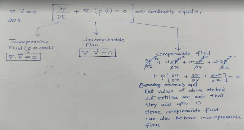
Incompressible flow means the volumetric strain rate of a flow is zero.It doesn't necessarily mean that fluid is compressible. The fluid can be compressible but still we can haveincompressible flow by maintaining volumetric strain rate equal to zero and having that desired values such that local and convective derivatives of density w.r.t time and space add up to zero. It is depicted mathematically in below figure.
Incompressible flow: div(velocity) = 0;
Incompressible fluid : ρ = constant;
Viscous flow means that there is resistance between two adjacent layers of fluid. Due to this resistance there is retardation of fluid flow. The cause of viscosity in liquids is due to cohesive forces whereas in gasses it is due to both molecular momentum exchange and cohesive forces.
Laminar flow occurs due to high viscous forces or low inertia forces. The criteria for laminar flow is defined by Reynolds number which is dimensionless and given by Re = Inertia force / Viscous force.
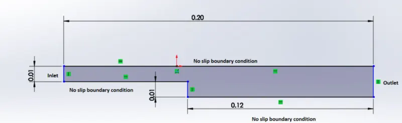
Now coming to the geometry of our problem through which fluid is going to flow. The geometry is known as backward facing step , which means that when the fluid is flowing in forward direction through the channel and there is step in between the path of fluid which leads to abrupt geometry change (sudden increase in flow area). This type of geometry in which there is abrupt change in flow area is known as backward facing step. It doesn't necessarily mean that there should be physical change in geometry , there can be cases where geometry is the same throughout but due to change in flow area there arises a backward facing step type of problem which is characterized by flow separation.The backward facing step problem is representation of flow separation problem which is widely seen in flow through airfoil, flow through ball, flow past a building, etc.
We will be having the below geometry for a fluid flow in this problem through which we will see how the flow separation occurs and what are the pressure values at which this thing occurs.
Procedure:
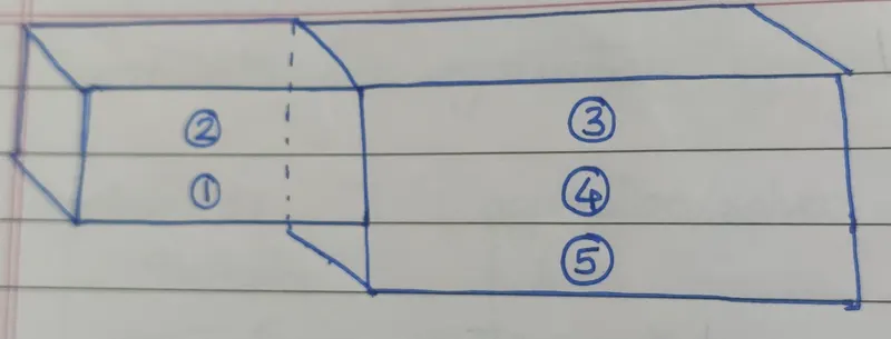
- Define the vertices and number of blocks on paper. In our case blocks are 5 and vertices are 22. We know how our geometry looks , we have to create the same geometry for the simulation.
- There is one folder in the tutorial folder which is provided by OpenFoam.We will copy that folder and paste it in run folder where all our simulations are carried out.It is to be noted that there are various case setups provided by the openFoam which are present in tutorial folder.
- Go into tutorial folder (type tut in terminal to navigate to tutorial folder), after this go to incompressible folder then into icoFoam folder After this go into cavity folder .
- Copy the cavity folder into the run folder by giving the following command. cp -r cavity/ $FOAM_RUN/ test. By typing these commands you will copy the cavity folder to the Run folder and rename it as test .
- Now navigate to the run folder by typing run in the terminal window.You will see the copied folder over here. Now inside the cavity folder you will see the list of folders which are common in all cases.
- In the system folder you will find the blockMeshdict file . Open this file by typing gedit blockMeshDict. We need to edit this file so that we can get our desired geometry.
- Define 22 vertices properly by following the right hand thumb rule whenever needed. After these define the blocks and the type of mesh along with the type of grading.Also define number of mesh points required in X,Y and Z direction. Here mesh points in x direction are 200, y direction are 20. I have defined total of 200 points in x direction block 1 and 2 having 80 mesh points and block 3 ,4 &5 having 120 mesh points. Similarly followed the same concept in y direction
- Now define the boundary condition as specified in the problem.
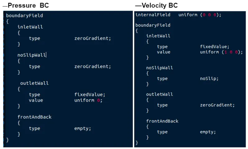
Here you have defined the geometry , now the next step is to set up the case by defining the physical properties, i.e;pressure and velocity. In this problem at inlet, velocity is constant and has a value of 1 m/s (assumed) in x direction whereas pressure is having zero gradient at inlet.
For outlet condition , the pressure is having fixed value whereas velocity is having zero gradient.The pressure value here is mentioned as 0 which denotes gauge pressure of the atmosphere.These two values can be edited by going into zero folder.
Now you can view our setup case, by typing paraFoam command in the test folder. This command will open ParaView where we will view our geometry.
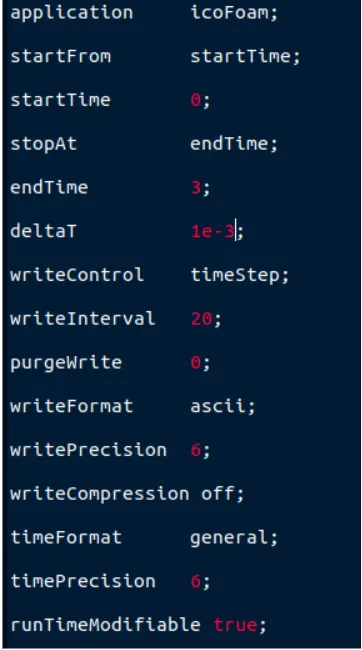
Now to run the simulation for our problem we need to define solver parameters in the controlDict file, Here we will define the start time , end time time for simulation and time interval between each solve.
CASE I : WITHOUT USING ANY GRADING FACTOR. (GF=1)
BLOCKMESDICT FILE
CODE:

Blockmeshdict:

/*--------------------------------*- C++ -*----------------------------------*\
  =========                 |
  \\      /  F ield         | OpenFOAM: The Open Source CFD Toolbox
   \\    /   O peration     | Website:  https://openfoam.org
    \\  /    A nd           | Version:  8
     \\/     M anipulation  |
\*---------------------------------------------------------------------------*/
FoamFile
{
    version     2.0;
    format      ascii;
    class       dictionary;
    object      blockMeshDict;
}
// * * * * * * * * * * * * * * * * * * * * * * * * * * * * * * * * * * * * * //

convertToMeters 1;

vertices
(
    (0 0 0)
    (0.08 0 0)
    (0.08 0.005 0)
    (0 0.005 0)
    (0.08 0.01 0)
    (0 0.01 0)
    (0.2 0.005 0)
    (0.2 0 0)
    (0.2 -0.01 0)
    (0.2 -0.01 0)
    (0.08 -0.01 0)

    (0 0 0.01)
    (0.08 0 0.01)
    (0.08 0.005 0.01)
    (0 0.005 0.01)
    (0.08 0.01 0.01)
    (0 0.01 0.01)
    (0.2 0.01 0.01)
    (0.2 0.005 0.01)
    (0.2 0 0.01)
    (0.2 -0.01 0.01)
    (0.08 -0.01 0.01)
);

blocks

(
    hex(0 1 2 3 11 12 13 14) (200 200 1) simpleGrading (1 1 1)
    hex(3 2 4 5 14 13 15 16) (200 200 1) simpleGrading (1 1 1)
    hex(2 7 6 4 13 18 17 15) (200 200 1) simpleGrading (1 1 1)
    hex(1 8 7 2 12 19 18 13) (200 200 1) simpleGrading (1 1 1)
    hex(10 9 8 1 21 20 19 12) (200 200 1) simpleGrading (1 1 1)
);

edges
(
);

boundary
(
inlet wall
{
type wall
faces
(
(11  14 3 0)
(14 16 5 3)
);
}

outlet wall
{
type wall
faces
(
(9 8 19 20)
(8 7 18 19)
(7 6 17 18)
);
}

frontandback
{
type empty
faces
(
(0 3 2 1)
(3 5 4 2)
(10 1 8 9)
(1 2 7 8)
(2 4 6 7)
(16 14 13 15)
(14 11 12 13)
(21 20 19 12)
(12 19 18 13)
(13 18 17 15)
);
}

noslipwall
{
type wall
faces
(
(4 5 16 15)
(4 15 17 6)
(0 1 12 11)
(9 20 21 10)
(1 10 21 12)
)
}
);


mergePatchPairs
(
);

// ************************************************************************* //
CONTROL DICT FILE:
/*--------------------------------*- C++ -*----------------------------------*\
  =========                 |
  \\      /  F ield         | OpenFOAM: The Open Source CFD Toolbox
   \\    /   O peration     | Website:  https://openfoam.org
    \\  /    A nd           | Version:  8
     \\/     M anipulation  |
\*---------------------------------------------------------------------------*/
FoamFile
{
    version     2.0;
    format      ascii;
    class       dictionary;
    location    "system";
    object      controlDict;
}
// * * * * * * * * * * * * * * * * * * * * * * * * * * * * * * * * * * * * * //

application     icoFoam;

startFrom       startTime;

startTime       0;

stopAt          endTime;

endTime         3;

deltaT          1e-3;

writeControl    timeStep;

writeInterval   20;

purgeWrite      0;

writeFormat     ascii;

writePrecision  6;

writeCompression off;

timeFormat      general;

timePrecision   6;

runTimeModifiable true;


// ************************************************************************* //
RESULTS:
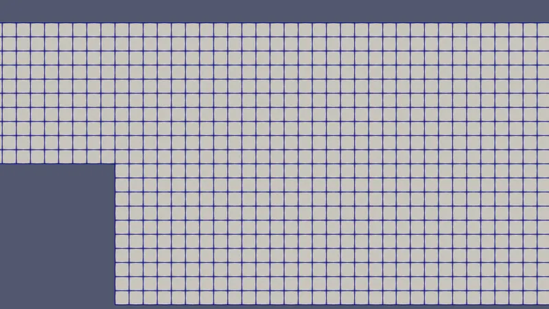
MESHED GEOMETRY

Detail view of mesh:
VELOCITY FLOW DISTRIBUTION:

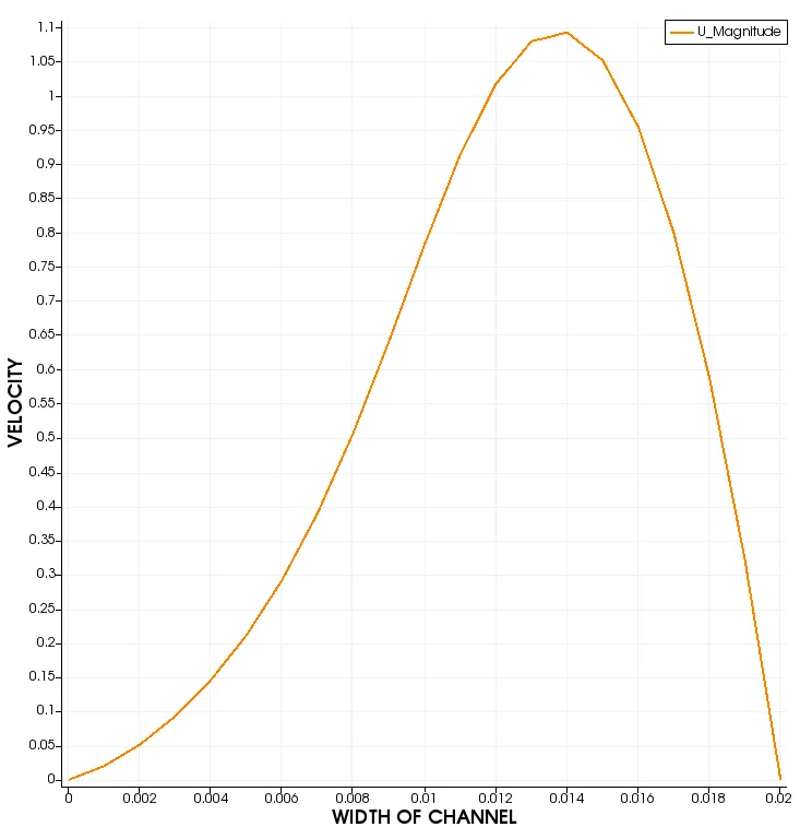
VELOCITY FLOW ALONG Y AXIS AT X=0.085m
CASE 2: WITH GRADING FACTOR = 0.2
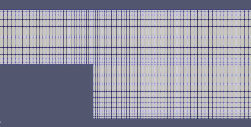
BLOCKMESHDICT FILE. In this case only grading factor is changed , other values of inlet condition are kept as it is. Also here as the mesh becomes finer the cell size decreases and hence Courants number increases. To avoid yhis we use smaller time interval value. Hence for finer mesh the simulation time will be more as compared to coarser mesh.
/*--------------------------------*- C++ -*----------------------------------*\
  =========                 |
  \\      /  F ield         | OpenFOAM: The Open Source CFD Toolbox
   \\    /   O peration     | Website:  https://openfoam.org
    \\  /    A nd           | Version:  8
     \\/     M anipulation  |
\*---------------------------------------------------------------------------*/
FoamFile
{
    version     2.0;
    format      ascii;
    class       dictionary;
    object      blockMeshDict;
}
// * * * * * * * * * * * * * * * * * * * * * * * * * * * * * * * * * * * * * //

convertToMeters 1;

vertices
(
     (0 0 0)
     (0.08 0 0)
     (0.08 0.005 0)
     (0 0.005 0)
     (0.08 0.01 0)
     (0 0.01 0)
     (0.2 0.01 0)
     (0.2 0.005 0)
     (0.2 0 0)
     (0.2 -0.01 0)
    (0.08 -0.01 0)

    (0 0 0.01)
    (0.08 0 0.01)
    (0.08 0.005 0.01)
    (0 0.005 0.01)
    (0.08 0.01 0.01)
    (0 0.01 0.01)
    (0.2 0.01 0.01)
    (0.2 0.005 0.01)
    (0.2 0 0.01)
    (0.2 -0.01 0.01)
    (0.08 -0.01 0.01)
);

blocks

(
    hex (0 1 2 3 11 12 13 14) (80 5 1) simpleGrading (0.2 5 1)
    hex (3 2 4 5 14 13 15 16) (80 5 1) simpleGrading (0.2 0.2 1)
    hex (2 7 6 4 13 18 17 15) (120 5 1) simpleGrading (5 0.2 1)
    hex (1 8 7 2 12 19 18 13) (120 5 1) simpleGrading (5 5 1)
    hex (10 9 8 1 21 20 19 12) (120 10 1) simpleGrading (5 5 1)
);

edges
(
);

boundary
(
inletWall
{
type patch;
faces
(
(11  14 3 0)
(14 16 5 3)
);
}

outletWall
{
type patch;
faces
(
(9 8 19 20)
(8 7 18 19)
(7 6 17 18)
);
}

frontAndBack
{
type empty;
faces
(
(0 3 2 1)
(3 5 4 2)
(10 1 8 9)
(1 2 7 8)
(2 4 6 7)
(16 14 13 15)
(14 11 12 13)
(21 20 19 12)
(12 19 18 13)
(13 18 17 15)
);
}

noSlipWall
{
type wall;
faces
(
(4 5 16 15)
(4 15 17 6)
(0 1 12 11)
(9 20 21 10)
(1 10 21 12)
);
}
);


mergePatchPairs
(
);

// ************************************************************************* //
Controldict File:
/*--------------------------------*- C++ -*----------------------------------*\
  =========                 |
  \\      /  F ield         | OpenFOAM: The Open Source CFD Toolbox
   \\    /   O peration     | Website:  https://openfoam.org
    \\  /    A nd           | Version:  8
     \\/     M anipulation  |
\*---------------------------------------------------------------------------*/
FoamFile
{
    version     2.0;
    format      ascii;
    class       dictionary;
    location    "system";
    object      controlDict;
}
// * * * * * * * * * * * * * * * * * * * * * * * * * * * * * * * * * * * * * //

application     icoFoam;

startFrom       startTime;

startTime       0;

stopAt          endTime;

endTime         3;

deltaT          1e-4;

writeControl    timeStep;

writeInterval   20;

purgeWrite      0;

writeFormat     ascii;

writePrecision  6;

writeCompression off;

timeFormat      general;

timePrecision   6;

runTimeModifiable true;


// ************************************************************************* //
RESULTS
Mesh details

Velocity distribution:

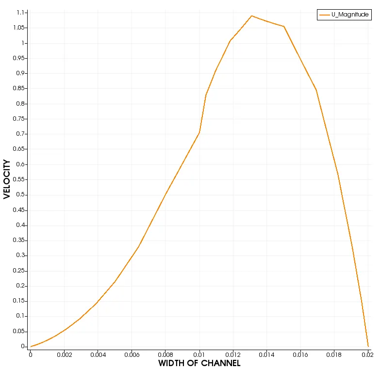
Velocity distribution along Y axis at 0.085m.
Conclusion:
With the use of GF , we observe that simulation time for later case is more as compared to case 1. This is because of finer mesh size which in term affects the CFL number. Hence we use higher dt value. Also the graph which we have plotted at 0.085m in both the cases,it is just after the flow sepearation and we can see that velocity is maximum at step region; around 1.092 m/s.
As we increase the finese of the mesh size the solution will become more accurate but we have to take care that CFL should not become high. Also the simulation time will also increase and hence computiong power required is more .