Week 9 - FVM Literature Review

Discretization principles:

1. Divide the domain into a number of discrete sub-domains,each sub-domain being represented by a number of discrete points.

2.Derive algebraic equation from the general differential equation ,valid at these discrete points.

3.Solve the system of algebraic equations to obtain values of the dependent variable at the discrete points.

Above three steps are common in the Finite Volume Method,Finite Difference Method and Finite Element Method.

Finite Difference Method :

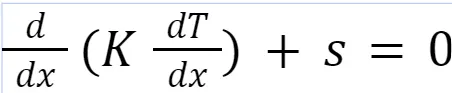
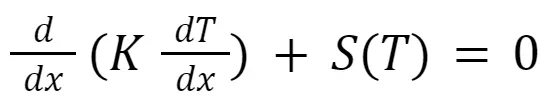
In FDM we divide the domain of interest into subdomain. After these we express the derivatives in terms of algebraic expression by using taylor series expansion.Consider a 1D steady state heat conduction equation:

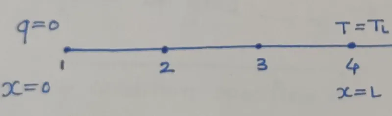
Now discretize the above equation by using a central differencing scheme about point 2. Note that the discrete points do not resemble any physical meaning w.r.t geometry, i.e these are arbitrary points.The length between each discrete points is assumed to be equal.

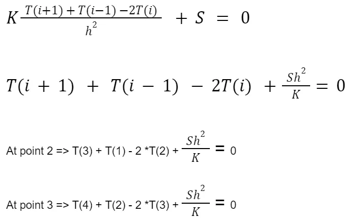
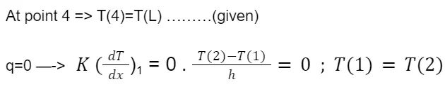
By following the above steps we get the values of dependent variable at the grid point. Here the dependent variable is Temperature (T).In FDM , the process of getting the algebraic equation and then applying boundary conditions to get the values at discrete points is very simple. One just need to follow the taylor series method to apply the suitable differencing schemes.

But,we see that for complex geometry discretization is difficult and hence capturing of real geometry from discretization becomes difficautand this may result in inaccuracy.Also in taylor series expansion we truncate the higher order terms , considering h —>0, but the derivative f’(x) , f’’(x) cannot be neglected.This leads to discrepancies in taylor series expansion and hence value of function will also change. This is the main drawback of FDM.

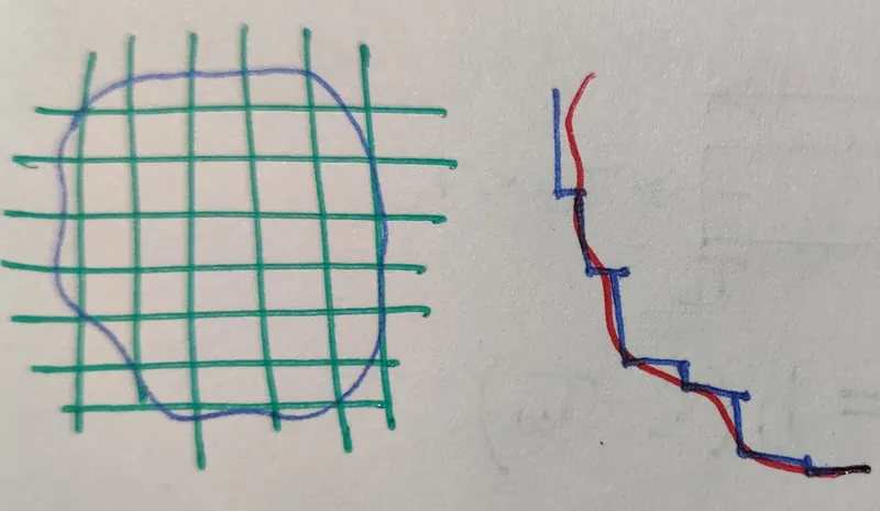
After the process of discretization, there are 2 things which should be expected from discretization.

1. Conservativeness: if the physical problem involves conservation of variable then its discretized variation should also conserve the variable.

Σ (conservation of discrete variable) = Domain conservation

FDM does not guarantee conservativeness.

2.Boundedness: For the temperature distribution in rod with no heat generation and steady state , one should expect that i in between the rod the temperature should not <0 C and >100C;i.e after discretization the solution should automatically come out which ensures this boundedness. So in FDM we hae not ensured this while discretizing the domain.

Finite Volume Method:

In FVM , there are three steps :

Step 1 :

Divide the domain into a number of finite size sub domains (control volume). Each sub domain is represented by a finite number of grid points.

Step 2:

Integrate the governing differential equation over each sub domain.

Step 3:

Consider a profile assumption for the dependent variable for evaluating the above integrals, to express the algebraic quantities at grid points.

Consider a similar example of 1D steady state heat conduction with variable heat source.

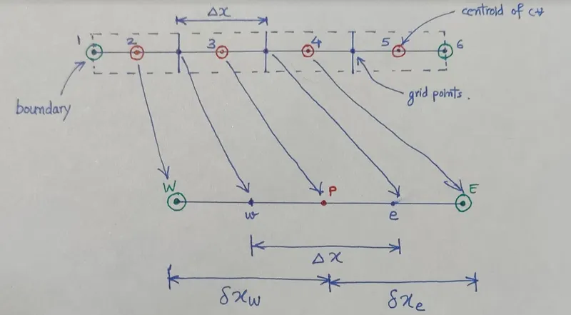
The rod is divided into 4 sub domains (control volume). Focusing on one control volume,the centroid is denoted by point P, the centroid present on the right side is denoted by E(east) and centroid present on the left side is denoted by W(west).. The boundary adjacent to east control volume is denoted by e and west is represented by w.

Now integrate the governing differential equation.

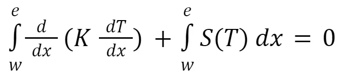
Consider S varies linearly with temperature T, i.e ; S=a+bT

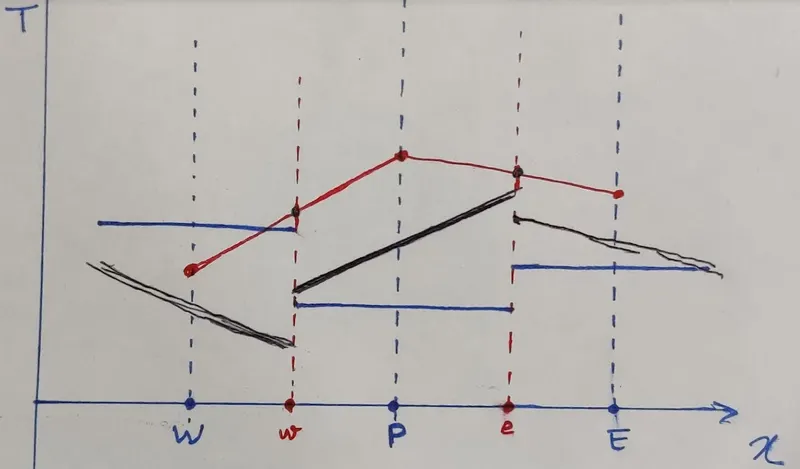
Now to evaluate the above equation we need to assume a profile for dependent variable.Here dependent variable is Temperature,T. The most obvious temperature profile is that of constant temperature. Now we need to dT/dx at the interface. So for the constant variation of temperature, dT/dx becomes 0.

But we know that heat flux is present due to which heat flow is happening.So now assuming piecewise linear variation of temperature between each control volume.Here also we see that dT/dx is discontinuous at faces,but one knows that heat flux is continuous.Hence piecewise linear variation for CV is not valid. But if we consider the piecewise linear profile between the grid points,then (dT/dx)e and (dT/dx)w are continuous.

For the source term we are assuming linear variation with temperature. Here temperature variation is assumed to be constant and has value of temperature at point P.

Now evaluating the above equation we get;

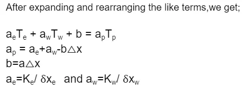
So the discretized equation follows conservatives and boundedness both as expected.

The main idea behind the construction of flux limiter schemes is to limit the spatial derivatives to realistic values—for scientific and engineering problems, this usually means physically realizable values. They are used in high-resolution schemes for solving problems described by PDEs and only come into operation when sharp wave fronts are present. For smoothly changing waves, the flux limiters do not operate and the spatial derivatives can be represented by higher-order approximations without introducing nonreal oscillations.