Week 3.5 - Deriving 4th order approximation of a 2nd order derivative using Taylor Table method
Objective: To derive the fourth order approximation for second order derivative and then compare the order of error for the given function w.r.t analytical derivative.
Theory: We will derive the fourth order approximation for second order derivative using following schemes
1) central differencing
2) right skewed
3) left skewed
Deriving using central differencing:
In central differencing, we take information from 4 neighbouring points; 2 of which are from right and other 2 from left.The stencil of the fourth order approximation looks like following
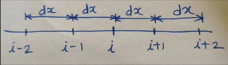
Based on the above stencil, we can write our expression as;
do^2(f)/do(x)^2=a*f(i-2)+b*f(i-1)+c*f(i)+d*f(i+1)+e*f(i+2).......(I)
Here our aim is to find a,b,c,d,e.Now we will use taylor table to get the 5 equations since we have 5 unknowns.
| f(i) | f'(i) dx | f''(i) dx^2 | f'''(i)*dx^3 | f""(i)*dx^4 | |
| a*f(i-2) | a | -2a | 4a/2 | 8a/6 | 16a/24 |
|
b*f(i-1) |
b | -b | b/2 | -b/6 | b/24 |
| c*f(i) | c | 0 | 0 | 0 | 0 |
| d*f(i+1) | d | d | d/2 | d/6 | d/24 |
| e*f(i+2) | e | 2e | 4e/2 | 8e/6 | 16e/24 |
| summation of 1st column | 0 | 0 | 1 | 0 | 0 |
After the formation of table you will get 5 equations as follows which are summation of each column ;
a+b+c+d+e=0..........(1)
2a+b-d-2e = 0..........(2)
4a/2+b/2+d/2+4e/2=1.......(3)
8a/6-b/6+d/6+8e/6=0........(4)
16a/24+b/24+d/24+16e/24=0...(5)
Now the above equations can be put up in matrix form of AX=B and then we can get the values of the coefficients.
a=-0.0833
b=1.333
c=-2.5
d=1.333
e=-0.0833
Now put these coefficients in equation (I) and you will get the formula for fourth order approximation of second order derivative by central differencing
Deriving using Right skewed :
In right skewed scheme we take information from right side of our point. The stencil for this scheme is shown below
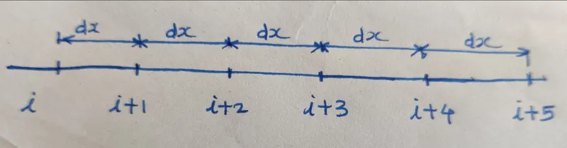
Based on the above stencil, we can write our expression as;
do^2(f)/do(x)^2=a*f(i)+b*f(i+1)+c*f(i+2)+d*f(i+3)+e*f(i+4)+F*f(i+5)......(II)
| f(i) | f'(i) *dx | f"(i)*dx^2 | f'''(i)*dx^3 | f''''(i)*dx^4 | f'''''(i)*dx^5 | |
| a*f(i) | a | 0 | 0 | 0 | 0 | 0 |
| b*f(i+1) | b | b | b/2 | b/6 | b/24 | b/120 |
| c*f(i+2) | c | 2c | 4c/2 | 8c/6 | 16c/24 | 32c/120 |
| d*f(i+3) | d | 3d | 9d/2 | 27d/6 | 81d/24 | 243d/120 |
| e*f(i+4) | e | 4e | 16e/2 | 64e/6 | 256e/24 | 1024e/120 |
| F*f(i+5) | F | 5F | 25F/2 | 125F/6 | 625F/24 | 3125F/120 |
| summation of all columns | 0 | 0 | 1 | 0 | 0 | 0 |
After the formation of table you will get 6 equations and we have 6 unknowns , so these can be solved by using matrices ; put the below 6 equations in matrix equation of AX=B
a+b+c+d+e+F=0.......(1)
b+2c+3d+4e+5F=0.....(2)
b/2+4c/2+9d/2+16e/2+25F/2=1....(3)
b/6+8c/6+27d/6+64e/6+125F/6=0...(4)
b/24+16c/24+81d/24+256e/24+625F/24...(5)
b/120+32c/120+243d/120+1024e/120+3125F/120=0....(6)
a=3.75
b=-12.833
c=17.833
d=-13
e=5.0833
F=-0.8333
Now put these coefficients in equation (II) and you will get the formula for fourth order approximation of second order derivative by right skewed scheme.
Deriving using left skewed
In left skewed scheme we take information from left side of our point. The stencil for this scheme is shown below
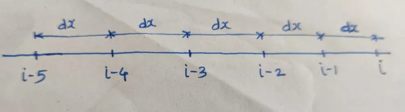
Based on the above stencil, we can write our expression as;
do^2(f)/do(x)^2=a*f(i-5)+b*f(i-4)+c*f(i-3)+d*f(i-2)+e*f(i-1)+F*f(i)......(III)
| f(i) | f'(i) | f"(i) | f'''(i) | f""(i) | f""'(i) | |
| a*f(i-5) | a | -5a | 25a/2 | -125a/6 | 625a/24 | -3125a/120 |
| b*f(i-4) | b | -4b | 16b/2 | -64b/6 | 256b/24 | -1024b/120 |
| c*f(i-3) | c | -3c | 9c/2 | -27c/6 | 81c/24 | -243c/120 |
| d*f(i-2) | d | -2d | 4d/2 | -8d/6 | 16d/24 | -32d/120 |
| e*f(i-1) | e | -e | e/2 | -e/6 | e/24 | -e/120 |
| F*f(i) | F | 0 | 0 | 0 | 0 | 0 |
| summation of all columns | 0 | 0 | 1 | 0 | 0 | 0 |
After the formation of table you will get 6 equations and we have 6 unknowns , so these can be solved by using matrices ; put the below 6 equations in matrix equation of AX=B
a+b+c+d+e+F=0
-5a-4b-3c-2d-e=0
25a/2+16b/2+9c/2+4d/2+e/2=1
-125a/6-64b/6-27c/6-8d/6-e/6=0
625a/24+256b/24+81c/24+16d/24+e/24=0
-3125a/120-1024b/120-243c/120-32d/120-e/120=0
a=-0.833
b=5.0833
c=-13
d=17.833
e=-12.833
F=3.75
Now put these coefficients in equation (III) and you will get the formula for fourth order approximation of second order derivative by left skewed scheme.
MATLAB CODE TO EVALUATE f(x)=(exp^x)*cos(x) by using 4th order approximations and compare the errors
%f(x)=(exp^x)*cos(x)
%analytical derivative

x=pi/3;
dx=linspace(pi/4,pi/40,40);

for i=1:length(dx)
    dx(i)

    %analytical derivative
    analytical_derivative = (-2)*exp(x)*sin(x)

%CENTRAL DIFFERENCING SCHEME
%coefficient value from taylor table
a= -0.083333;
b= 1.333333;
c= -2.5000;
d= 1.333333;
e= -0.083333;

central_diff_approx(i) = ((a*exp(x-2*dx(i))*cos(x-2*dx(i)))+(b*exp(x-dx(i))*cos(x-dx(i)))+(c*exp(x)*cos(x))+(d*exp(x+dx(i))*cos(x+dx(i)))+(e*exp(x+2*dx(i))*cos(x+2*dx(i))))/dx(i)^2
central_diff_error(i)=abs(central_diff_approx(i)-analytical_derivative)

%RIGHT SKEWED DIFERENCING SCHEME
%coefficient value from taylor table
a=3.75000;
b=-12.8333;
c=17.8333;
d=-13.000;
e=5.08333;
f=-0.8333;

right_skewed_approx(i)=((a*exp(x)*cos(x))+(b*exp(x+dx(i))*cos(x+dx(i)))+(c*exp(x+2*dx(i))*cos(x+2*dx(i)))+(d*exp(x+3*dx(i))*cos(x+3*dx(i)))+(e*exp(x+4*dx(i))*cos(x+4*dx(i)))+(f*exp(x+5*dx(i))*cos(x+5*dx(i))))/dx(i)^2
right_skewed_error(i)=abs(right_skewed_approx(i)-analytical_derivative)

%LEFT SKEWED DIFFERENCING SCHEME
%coefficient value from taylor table
a= -0.8333;
b= 5.08333;
c= -13.0000;
d= 17.8333;
e= -12.8333;
f= 3.75000;

left_skewed_approx(i)=((a*exp(x-5*dx(i))*cos(x-5*dx(i)))+(b*exp(x-4*dx(i))*cos(x-4*dx(i)))+(c*exp(x-3*dx(i))*cos(x-3*dx(i)))+(d*exp(x-2*dx(i))*cos(x-2*dx(i)))+(e*exp(x-dx(i))*cos(x-dx(i)))+(f*exp(x)*cos(x)))/dx(i)^2
left_skewed_error(i)=abs(left_skewed_approx(i)-analytical_derivative)

end


figure(1)
plot(dx,central_diff_error,'g','linewidth',2)
hold on
plot(dx,right_skewed_error,'red','linewidth',2)
hold on
plot(dx,left_skewed_error,'y','linewidth',2)
legend('central diff error','right skewed error','left skewed error')


figure(2)
loglog(dx,central_diff_error,'g','linewidth',2)
hold on
loglog(dx,right_skewed_error,'red','linewidth',2)
hold on
loglog(dx,left_skewed_error,'y','linewidth',2)
legend('central diff error','right skewed error','left skewed error')
Plot of dx v/s error LOG-LOG PLOT OF dx v/s error
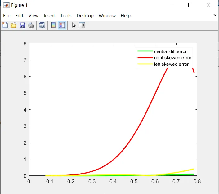
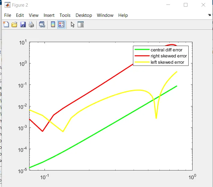
Conclusion: After seeing the plot we can conclude that central differencing produces more accurate reults and hence less error than other two schemes.
Reason why skewed schemes is useful?
Central differencing scheme is useful when we are calculating the approximation of the function at a point which is at the centre of grid or the point has equal number of neighbouring points on both right and left. But what about the points in the grid which are at corner of the grid, we cannot use here central differencing hence Right/Left skewed difference scheme is used. So we can take data from one side of the point and calculate accordingly.