Week 7 - Simulation of a 1D Super-sonic nozzle flow simulation using Macormack Method
Objective: To simulate the isentropic flow through quasi 1D flow through subsonic-supersonic nozzle, by deriving conservation and non conservation forms of governing equations and solve them by using MacCormack’s technique.
Expected Results:
1.Determine the steady state temperature distribution of the flow field variables.
2.Variation of primitive variables w.r.t timesteps and along the length of nozzle.
3.Mass flow rate distribution inside the nozzle at different timesteps.
4.Compare normalized mass flow rate distribution of both forms.
Theory:
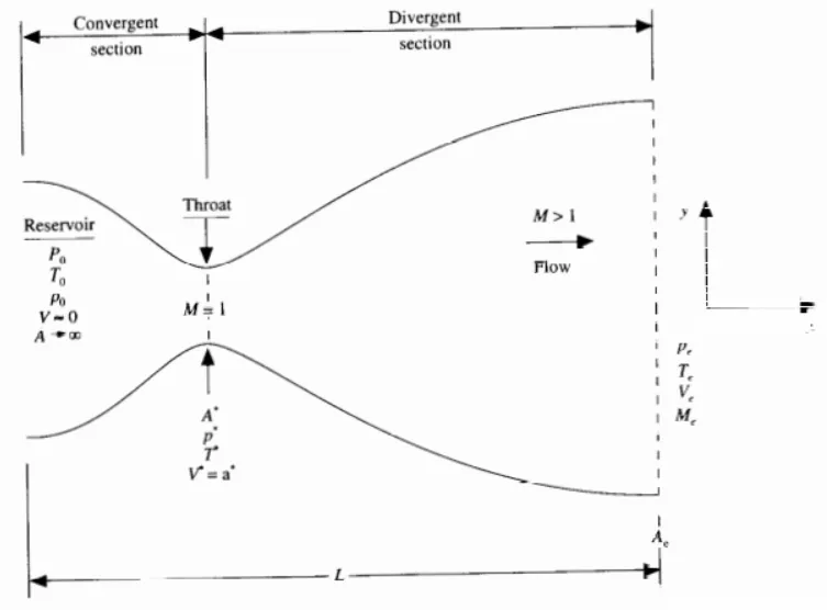
Here we consider the steady isentropic flow through the nozzle. The one end of the nozzle is attached to the reservoir,hence the entering velocity at inlet of the nozzle is assumed to be nearly equal to zero (as compared to outlet velocity and throat velocity). The area of nozzle is varying w.r.t to nozzle,hence it becomes a 2D flow problem.But we assume that flow properties do not vary in the y direction,i.e we neglect the effect of variation of flow properties in y direction. This type of problem is known as quasi 1D flow. This assumption leads to uniform flow properties across any given cross section.
As the one end of the nozzle is attached to the reservoir, the area,A tends to infinity hence velocity is nearly equal to 0. The properties at this point are known as stagnation properties, which are denoted as P0, T0 and ⍴0 as denoted in below figure. The flow expands isentropically towards exit with value as Pe, Te and ⍴e .
Figure(1): schematic diag of nozzle.
A. Governing flow equation:
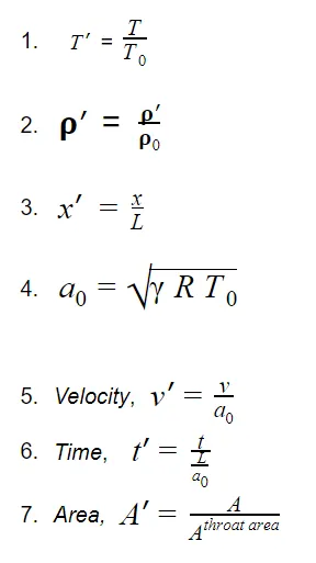
I. Non-dimensional primitive variables:
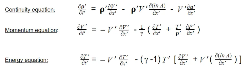
II. Non-conservation equation:
III. Conservation equation:
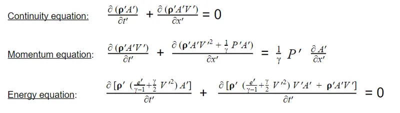
To write the conservation equation in general form,
Let Solution vector= U ,Flux vector= F and Source vector= J.
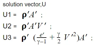
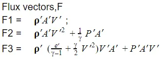
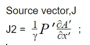
With the above equations, conservation equation can be written as;
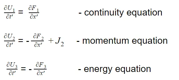
As the above equations are conservative form, here dependent variables are not primitive variables. After solving the above equation, we will get value for U1,U2 and U3. So we define define primitive variables in terms of U1,U2,U3 .
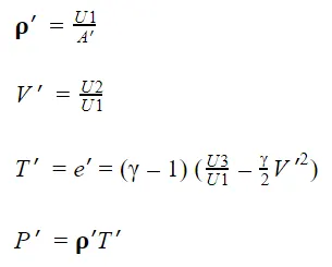
B. MATLAB CODE TO SOLVE THE GOVERNING EQUATIONS USING MacCormack's technique.
Now to solve the non-conservation and conservation equation numerically we will use MacCormack’s technique
The code to solve the above equations is divided into 3 parts,
Part 1: function for non conservation equation.
Part 2: function for conservation equation.
Part 3: Main code to solve above functions.
PART 1: MATLAB CODE FOR FUNCTION OF NON CONSERVATION EQUATION.
function[mass_flow_nonc,rho_nonc,v_nonc,T_nonc,M_nonc,P_nonc,rho_t_nonc,T_t_nonc,P_t_nonc,M_t_nonc]=non_conservation(n,x,dx,gamma,A,C,nt)


%defining domain
n=31;
x=linspace(0,3,n);
dx=x(2)-x(1);

%boundary conditions
rho_nonc=1-0.3146.*x;                    %density
T_nonc=1-0.2314.*x;                      %temperature
v_nonc=(0.1+1.09*x).*T_nonc.^0.5;        %velocity
gamma=1.4;

%area profile
A=1+2.2*(x-1.5).^2;

figure(2)
plot(A)
throat=find(A==1);

nt=1400;


for k=1:nt


    rho_old=rho_nonc;
    v_old=v_nonc;
    T_old=T_nonc;

    %time step
    B=(T_nonc.^0.5);
    dt=C.*(dx./((B)+v_nonc));
    dt=min(dt);

    %predictor method
    for j=2:n-1
        dvdx=(v_nonc(j+1)-v_nonc(j))/dx;
        drhodx=(rho_nonc(j+1)-rho_nonc(j))/dx;
        dTdx=(T_nonc(j+1)-T_nonc(j))/dx;
        dlogAdx=(log(A(j+1))-log(A(j)))/dx;

        %continuity equation
        drhodt_p(j)=-rho_nonc(j)*(dvdx)-rho_nonc(j)*v_nonc(j)*dlogAdx-v_nonc(j)*drhodx;

        %momentum equation
        dvdt_p(j)=-v_nonc(j)*(dvdx)-(1/gamma)*(dTdx+(T_nonc(j)/rho_nonc(j))*drhodx);

        %energy equation
        dTdt_p(j)=-v_nonc(j)*(dTdx) - (gamma-1)*T_nonc(j)*(dvdx + v_nonc(j)*dlogAdx);

        %solution update
         rho_nonc(j)=rho_nonc(j) + drhodt_p(j)*dt;
         v_nonc(j)=v_nonc(j) + dvdt_p(j)*dt;
         T_nonc(j)=T_nonc(j) + dTdt_p(j)*dt;

    end

    %corrector method
    for j=2:n-1
        dvdx=(v_nonc(j)-v_nonc(j-1))/dx;
        drhodx=(rho_nonc(j)-rho_nonc(j-1))/dx;
        dTdx=(T_nonc(j)-T_nonc(j-1))/dx;
        dlogAdx=(log(A(j))-log(A(j-1)))/dx;

        %continuity equation
        drhodt_c(j)=-rho_nonc(j)*(dvdx)-rho_nonc(j)*v_nonc(j)*(dlogAdx)- v_nonc(j)*drhodx;

        %momentum equation
        dvdt_c(j)=-v_nonc(j)*(dvdx)-(1/gamma)*((dTdx)+(T_nonc(j)/rho_nonc(j))*drhodx);

        %energy equation
        dTdt_c(j)=-v_nonc(j)*(dTdx) - (gamma-1)*T_nonc(j)*(dvdx + v_nonc(j)*dlogAdx);

    end
        %computing the average time derivative
        drhodt = 0.5*(drhodt_p + drhodt_c);
        dvdt   = 0.5*(dvdt_p + dvdt_c);
        dTdt  = 0.5*(dTdt_p+ dTdt_c);

        %final solution update

        for i = 2:n-1
            rho_nonc(i)= rho_old(i)+drhodt(i)*dt;
            v_nonc(i)=  v_old(i)+dvdt(i)*dt;
            T_nonc(i)=  T_old(i)+dTdt(i)*dt;
        end


        %apply the boundary conditions

        %inlet
        v_nonc(1)=2*v_nonc(2)-v_nonc(3);

        %outlet
        v_nonc(n)=2*v_nonc(n-1)-v_nonc(n-2);
        rho_nonc(n)=2*rho_nonc(n-1)-rho_nonc(n-2);
        T_nonc(n)=2*T_nonc(n-1)-T_nonc(n-2);

        M_nonc=v_nonc./(T_nonc.^0.5);
        P_nonc=rho_nonc.*T_nonc;
        mass_flow_nonc=rho_nonc.*v_nonc.*A;

        %PLOTTING MASS FLOW RATE

    rho_t_nonc(k)=rho_nonc(throat);
    T_t_nonc(k)=T_nonc(throat);
    v_t_nonc(k)=v_nonc(throat);
    mass_flow_t_nonc(k)=mass_flow_nonc(throat);
    P_t_nonc(k)=P_nonc(throat);
    M_t_nonc(k)=M_nonc(throat);

        figure(3)

        if k==50
            plot(x,mass_flow_nonc,'color','g','linewidth',1.5)
            hold on
        elseif k==100
            plot(x,mass_flow_nonc,'color','yellow','linewidth',1.5)
            hold on
        elseif k==200
            plot(x,mass_flow_nonc,'color','blue','linewidth',1.5)
            hold on
        elseif k==400
            plot(x,mass_flow_nonc,'color','magenta','linewidth',1.5)
            hold on
        elseif k==800
            plot(x,mass_flow_nonc,'color','red','linewidth',1.5)
            hold on
        elseif k==1400
            plot(x,mass_flow_nonc,'color','k','linewidth',1.5)
            hold on
        end

    title('MASS FLOW RATES AT DIFFERENT TIMESTEPS-NON CONSERVATION FORM')
    xlabel('Distance')
    ylabel('Mass flow rate')
    legend("50th timestep","100th timestep","200th timestep","400th timestep","800th timestep","1400th timestep")
    grid on

    end
Code explaination:
1. The function is defined by the name non_conservation with output variables as mass flow rate , velocity , density , temperature, pressure and Mach number in the nozzle and at throat (t).
2. The domain is defined with grid points ,n=31 ,divided over the length of 3m. Also the boundary condition and area profile of nozzle is defined. This values are taken from CFD book by John D. Anderson.
3. To make our soultion stable , a stability criteria is used, which is CFL<=0.5. From these value min time step value is defined, min(dt).
4. Next predictor step is used to get the predicted values of our primitive variables.
5. Similarly corrector step is used to get the corrected values. Atlast average time derivative value is calculated from predictor and corrector step. And finally the values for primitive variables are calculated for internal grid points; 2 to n-1.
6. Now we apply the boundary at inlet and outlet.
PART 2: MATLAB CODE FOR FUNCTION OF CONSERVATION EQUATION.
function[U1,U2,U3,mass_flow_con,rho,v,T,M,P,rho_t,T_t,v_t,P_t,M_t]=conservation(n,x,dx,gamma,A,C,nt)

n=31;
nt=1400;

for i=1:n
    if (x(i)>=0 && x(i)<=0.5)
        rho(i)=1;
        T(i)=1;
    elseif (x(i)>=0.5 && x(i)<=1.5)
        rho(i)=1-0.366*(x(i)-0.5);
        T(i)=1-0.167*(x(i)-0.5);
    elseif (x(i)>=1.5 && x(i)<=3.5)
        rho(i)=0.634-0.3879*(x(i)-1.5);
        T(i)=0.833-0.3507*(x(i)-1.5);
    end
end


%initial profile for area,velocity and pressure

A=1+2.2*(x-1.5).^2;
throat_c=find(A==1);
v=0.59./(rho.*A);
P=rho.*T;

%Initial solution vectors
U1=rho.*A;
U2=rho.*A.*v;
U3=rho.*A.*(T./(gamma-1))+((gamma/2)*v.^2);


for k=1:nt

    dt=min(C.*dx./(sqrt(T)+v));

    U1_old=U1;
    U2_old=U2;
    U3_old=U3;

    %calculating flux vectors
    F1=U2;
    F2=((U2.^2)./U1)+((gamma-1)/gamma)*(U3-(gamma/2)*(U2.^2)./U1);
    F3=((gamma*U2.*U3)./U1)-(gamma*(gamma-1)*((U2.^3)./(2*U1.^2)));

    %PREDICTOR METHOD

    for j=2:n-1

        J2(j)=(1/gamma)*rho(j)*T(j)*(A(j+1)-A(j))/(dx);

        %continuity equation
        dU1dt_p(j)=-(F1(j+1)-F1(j))/dx;

        %momentum equation
        dU2dt_p(j)=-((F2(j+1)-F2(j))/(dx))+J2(j);

        %energy equation
        dU3dt_p(j)=-((F3(j+1)-F3(j))/dx);

        %Updating new values

        U1(j)=U1(j)+dU1dt_p(j)*dt;
        U2(j)=U2(j)+dU2dt_p(j)*dt;
        U3(j)=U3(j)+dU3dt_p(j)*dt;
    end

    %updating flux vectors
    F1=U2;
    F2=((U2.^2)./U1)+((gamma-1)/gamma)*(U3-(gamma/2)*(U2.^2)./U1);
    F3=((gamma*U2.*U3)./U1)-(gamma*(gamma-1)*((U2.^3)./(2*U1.^2)));


    %CORRECTOR METHOD

    rho=U1./A;
    v=U2./U1;
    T=(gamma-1)*((U3./U1-(gamma/2)*(v).^2));

    for j=2:n-1

        J2(j)=(1/gamma)*rho(j)*T(j)*(A(j)-A(j-1))/(dx);

        %continuity equation
        dU1dt_c(j)=-(F1(j)-F1(j-1))/dx;

        %momentum equation
        dU2dt_c(j)=-((F2(j)-F2(j-1))/dx)+J2(j);

        %energy equation
        dU3dt_c(j)=-((F3(j)-F3(j-1))/dx);
    end

    %computing average time derivatives
    dU1dt=0.5*(dU1dt_p+dU1dt_c);
    dU2dt=0.5*(dU2dt_p+dU2dt_c);
    dU3dt=0.5*(dU3dt_p+dU3dt_c);

    %Final solution matrix

    for i=2:n-1

        U1(i)=U1_old(i)+dU1dt(i)*dt;
        U2(i)=U2_old(i)+dU2dt(i)*dt;
        U3(i)=U3_old(i)+dU3dt(i)*dt;

    end

   %Boundary conditions

    %At inlet

    U1(1)=rho(1)*A(1);
    U2(1)=2*U2(2)-U2(3);
    v(1)=U2(1)./U1(1);
    U3(1)=U1(1)*((T(1)/(gamma-1))+((gamma/2)*(v(1)).^2));

    %At Outlet

    U1(n)=2*U1(n-1)-U1(n-2);
    U2(n)=2*U2(n-1)-U2(n-2);
    U3(n)=2*U3(n-1)-U3(n-2);

    %Final Primitive value update

    rho=U1./A;
    v=U2./U1;
    T=(gamma-1)*((U3./U1-(gamma/2)*(v).^2));


    %mass flow rate
    %M=mach number

    mass_flow_con=rho.*A.*v;
    P=rho.*T;
    M=(v./sqrt(T));

    %THROAT VARIABLES

    rho_t(k)=rho(throat_c);
    T_t(k)=T(throat_c);
    v_t(k)=v(throat_c);
    mass_flow_con_t(k)=mass_flow_con(throat_c);
    P_t(k)=P(throat_c);
    M_t(k)=M(throat_c);

    %PLOT
    figure(3)

    if k==50
        plot(x,mass_flow_con,'k','linewidth',2);
        hold on
    elseif k==100
        plot(x,mass_flow_con,'g','linewidth',2);
        hold on
    elseif k==200
        plot(x,mass_flow_con,'r','linewidth',2);
        hold on
    elseif k==400
        plot(x,mass_flow_con,'m','linewidth',2);
        hold on
    elseif k==800
        plot(x,mass_flow_con,'y','linewidth',2);
        hold on
    elseif k==1400
        plot(x,mass_flow_con,'y','linewidth',2);
        hold on
    end

    title('MASS FLOW RATES AT DIFFERENT TIMESTEPS-CONSERVATION FORM')
    xlabel('Distance')
    ylabel('Mass flow rate')
    legend("50th timestep","100th timestep","200th timestep","400th timestep","800th timestep","1400th timestep")
end
end
Code explaination:
1. The function is defined by the name non_conservation with output variables as mass flow rate , velocity , density , temperature, pressure and Mach number in the nozzle and at throat (t).
2. The domain is defined with grid points ,n=31 ,divided over the length of 3m. Also the boundary condition and area profile of nozzle is defined. This values are taken from CFD book by John D. Anderson.
3. To make our soultion stable , a stability criteria is used, which is CFL<=0.5. From these value min time step value is defined, min(dt).
4. As the dependent variable in the conservation equation are U1,U2 and U3, there values are synthesized from initial conditions of density and temperature (non-dimensional).
5. Next we define the solution vectors and flux vectors. Here flux vectors are defined in terms of U1,U2 and U3.
6. After defining the boundary conditions, we use similar technique of predictor and corrector step for conservation equation.
PART 3: MAIN CODE
n=31;
gamma=1.4;
x=linspace(0,3,n);
dx=x(2)-x(1);
A=1+2.2*(x-1.5).^2;
nt=1400;
throat=find(A==1);


C=0.5; %courant number

%Calling non conservation function

tic;
[mass_flow_nonc,rho_nonc,v_nonc,T_nonc,M_nonc,P_nonc,rho_t_nonc,T_t_nonc,P_t_nonc,M_t_nonc]=non_conservation(n,x,dx,gamma,A,C,nt);
Time_taken_nonc=toc;
hold on

%PLOTTING Variation of properties at throat with number of timesteps
figure(4)

%DENSITY
subplot(4,1,1)
plot(linspace(1,nt,nt),rho_t_nonc,'k')
ylabel('DENSITY')
legend("DENSITY AT THROAT")
axis([0 1400 0 1.3])
title('Timestep variation at throat-NON CONSERVATION FORM')

%TEMPERATURE
subplot(4,1,2)
plot(linspace(1,nt,nt),T_t_nonc,'m')
ylabel('TEMPERATURE')
legend("TEMPERATURE AT THROAT")

%PRESSURE
subplot(4,1,3)
plot(linspace(1,nt,nt),P_t_nonc,'y')
ylabel('PRESSURE')
legend("PRESSURE AT THROAT")


%MACH NUMBER
subplot(4,1,4)
plot(linspace(1,nt,nt),M_t_nonc,'g')
ylabel('MACH NUMBER')
legend("MACH NUMBER AT THROAT")

%plotting variation of primitive variable with nozzle length
figure(5)

%DENSITY
subplot(4,1,1)
plot(x,rho_nonc,'k')
ylabel('Density')
legend("DENSITY")
axis([0 3 0 1])
grid on
title("PROPERTY VARIATION ALONG THE LENGTH OF NOZZLE")

%TEMPERATURE
subplot(4,1,2)
plot(x,T_nonc,'b')
ylabel('TEMPERATURE')
legend("TEMPERATURE")
axis([0 3 0 1])


%PRESSURE
subplot(4,1,3)
plot(x,P_nonc,'r')
ylabel('PRESSURE')
legend("PRESSURE")
axis([0 3 0 1])


%MACH NUMBER
subplot(4,1,4)
plot(x,M_nonc,'m')
ylabel('MACH NUMBER')
legend("MACH NUMBER")
axis([0 3 0 5])


%Calling conservation function
tic;
[U1,U2,U3,mass_flow_con,rho,v,T,M,P,rho_t,T_t,v_t,P_t,M_t]=conservation(n,x,dx,gamma,A,C,nt);
Time_taken_c=toc;
hold on


%PLOTTING Variation of properties at throat with number of timesteps
 figure(6)
Z=linspace(1,nt,nt);
%DENSITY
subplot(4,1,1)
plot(Z,rho_t,'k')
ylabel('DENSITY')
legend("DENSITY AT THROAT")
axis([0 1400 0 3])
title('Timestep variation at throat- CONSERVATION FORM')

%TEMPERATURE
subplot(4,1,2)
plot(Z,T_t,'m')
ylabel('TEMPERATURE')
legend("TEMPERATURE AT THROAT -CONSERVATION")

%PRESSURE
subplot(4,1,3)
plot(Z,P_t,'y')
ylabel('PRESSURE')
legend("PRESSURE AT THROAT -CONSERVATION")


%MACH NUMBER
subplot(4,1,4)
plot(Z,M_t,'g')
ylabel('MACH NUMBER')
legend("MACH NUMBER AT THROAT -CONSERVATION")

%plotting variation of primitive variable with nozzle length
figure(7)

%DENSITY
subplot(4,1,1)
plot(x,rho,'k')
ylabel('Density')
legend("DENSITY -CONSERVATION")
axis([0 3 0 1])
grid on
title("PROPERTY VARIATION ALONG THE LENGTH OF NOZZLE-CONSERVATION")

%TEMPERATURE
subplot(4,1,2)
plot(x,T,'b')
ylabel('TEMPERATURE')
legend("TEMPERATURE -CONSERVATION")
axis([0 3 0 1])


%PRESSURE
subplot(4,1,3)
plot(x,P,'r')
ylabel('PRESSURE')
legend("PRESSURE -CONSERVATION")
axis([0 3 0 1])


%MACH NUMBER
subplot(4,1,4)
plot(x,M,'m')
ylabel('MACH NUMBER')
legend("MACH NUMBER -CONSERVATION")
axis([0 3 0 5])


%COMPARISON OF MASS FLOW RATES
figure(8)

plot(x,mass_flow_nonc,'r','linewidth',1.2)
hold on
plot(x,mass_flow_con,'k','linewidth',1.25)
hold off

grid on
Results:
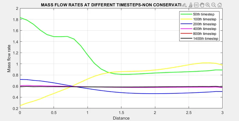
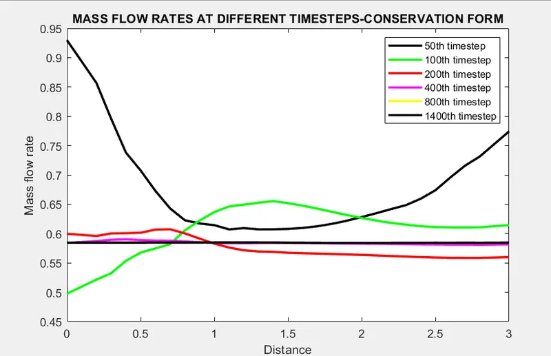
I. Mass flow rate variation inside the nozzle at different time steps.
Observation:
In both of the forms of equation we can see that mass flow rate becomes steady after 400 timesteps.
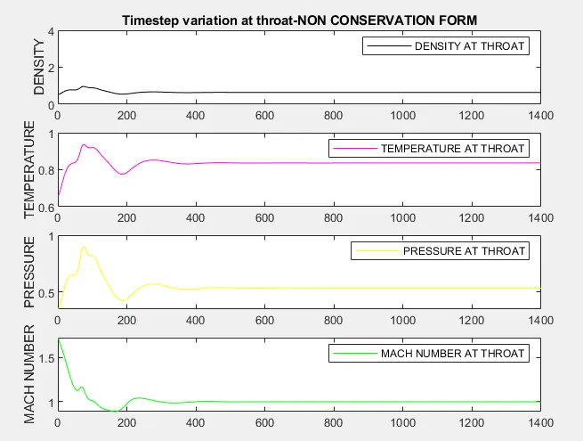
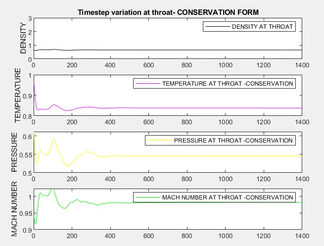
II. Variation of properties at throat with number of time steps.
Observation:
Here we see that the value of primitive variables in non conservation equation becomes steady after a while as compared to conservation equation. This can be inferred from the above figure.
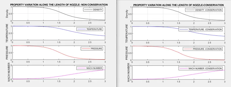
III. Variation of properties along the length of nozzle
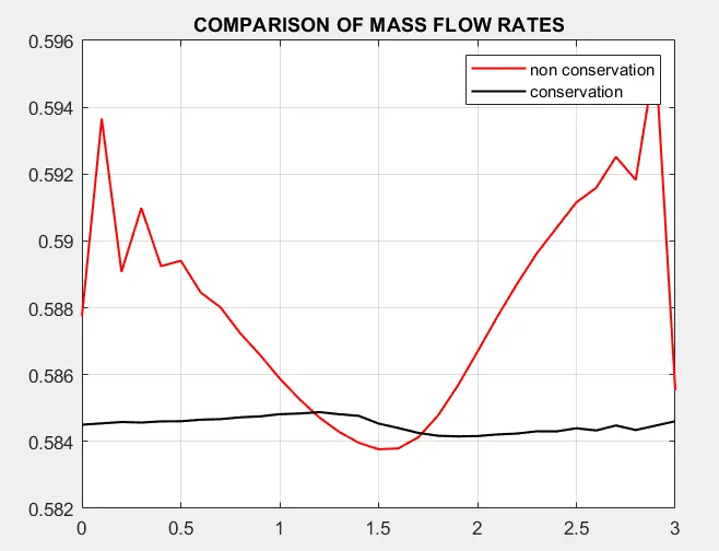
IV. Comparison of mass flow rate in both forms of equation
Observation
The graph for non-conservation oscillates more than the conservation graph. Here the mass flow rate is constant with a value of around 0.579. The conservation graph being more closer to being constant matches the exact solution. Although the distribution in above figure have been magnified for more clarity. We can see that the variation in non-conservation comes at inlet and outlet of nozzle.
Grid dependence test:

After changing the grid points from n=31 to 61 we see that at the end of 1400th timestep; the values of primitive variable do not change much. Here we can infere that given problem is grid independent. This test helps us to decrease the simulation time by keeping the values of the variables same.
Conclusion:
1. From the comparison of mass flow rate figure , we conclude that conservation equation gives value closer to exact value. Here conservation equation does better job.
2. The result for primitive variables by non conservation equation are more accurate than its counter part. However the values for flux terms are slightly more accurate by conservation form.
3. To write the code for conservation form requires more effort, first we have to define solution vectors in terms of primitive variables ,then define flux vectors in terms of solution vector and then finally solve the equation. This all is not required in non-conservation form.
4. Although both th form of equation can be used inter dependent on one another, and one can be derived from other. But while solving the problem each one of them has there own pros and cons. Here conservation equation yields faster result as compared to non conservation . In terms of values of primitive variables non conservation does better job. And in terms of complexity of solution , conservation equation is more complex than non conservation.