Week 5.1 - Mid term project - Solving the steady and unsteady 2D heat conduction problem
Title: Solving steady and unsteady 2d heat conduction equation by using iterative solvers.
Theory:
The square plate of unit thickness is subjected to various temperatures which are given below
Temp at top=600 K
Temp at bottom=900K
Temp at left= 400K
Temp at right= 800K
Assumptions:
1.Plate is homogeneous and isotropic i.e alpha ≠f(x,y,t).
2.No heat generation in plate.
3. 2d heat conduction.
4. No convection is present.
The 2d general heat conduction without heat generation is given as:
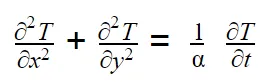
A. For steady state the equation is given as:
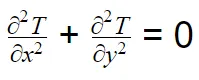
The above equation can be solved by numerical discretization:

Solving for T(i,j),we get;
 .....................(1)
where K is given as below
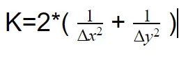
Now to solve the equation (1),we will use various iterative methods,
1)Jacobi method
2)Gauss-siedal method
3)Successive over relaxation method
Matlab code for 2d steady state heat conduction equation
clear all
close all
clc

%given boundary condition
T_top=600;
T_bottom=900;
T_left=400;
T_right=800;

%defining grid points
nx=51;
x=linspace(0,1,nx);
dx=x(2)-x(1);
ny=nx;
y=linspace(0,1,ny);
dy=y(2)-y(1);
T=300*ones(nx,ny);

T(:,end)=T_right;                      %temp at right
T(:,1)=T_left;                         %temp at right
T(1,:)=T_top;                          %temp at top
T(end,:)=T_bottom;                     %temp at bottom

%CORNER TEMPERATURES
T(end,end)=(T_bottom+T_right)/2;
T(1,end)=(T_top+T_right)/2;
T(1,1)=(T_top+T_left)/2;
T(end,1)=(T_bottom+T_left)/2;
k=2*(1/(dx)^2 + (1/(dy)^2));


tol=1e-5;
error=9e9;
T_old=T;


iterative_solver=1               %  enter 1 for jacobi_method
                                 %  enter 2 for Gauss_siedal_method
                                 %  enter 3 for sor


if iterative_solver ==1  %jacobi method
    jacobi_iter=0;

    while(error>tol)
        for i=2:nx-1
            for j=2:ny-1
                T(i,j)=((T_old(i+1,j)+T_old(i-1,j))/(dx)^2 )/k+ ((T_old(i,j+1)+T_old(i,j-1))/(dy)^2)/k ;
            end
            error=max(max(abs(T-T_old)));
            T_old=T;
            jacobi_iter=jacobi_iter+1;

        end
    end
    figure(1)
    C = contourf(x,y,T,'ShowText','on');
    xlabel('x')
    ylabel('y')
    set(gca,'YDIR','reverse')
    colormap(jet)
    title_text=sprintf('No of iterations Jacobi = %d',jacobi_iter);
    title(title_text)

end


if iterative_solver ==2   %Gauss siedal method
    Gauss_siedal_iter=0;

    while(error>tol)
        for j=2:ny-1
            for i=2:nx-1
                T(i,j)=((T_old(i+1,j)+T(i-1,j))/(dx)^2 )/k+ ((T_old(i,j+1)+T(i,j-1))/(dy)^2)/k ;

            end
            error=max(max(abs(T-T_old)));
            T_old=T;
            Gauss_siedal_iter=Gauss_siedal_iter+1;

        end
    end
    figure(2)
    C = contourf(x,y,T,'ShowText','on');
    xlabel('x')
    ylabel('y')
    set(gca,'YDIR','reverse')
    colormap(jet)
    title_text=sprintf('No of iterations GS = %d',Gauss_siedal_iter);
    title(title_text)
end


if iterative_solver ==3  %sor method
    beta=1.8;
    sor_iter=0;

    while(error>tol)
        for j=2:ny-1
            for i=2:nx-1
                T(i,j)=((T_old(i+1,j)+T(i-1,j))/(dx)^2 )/k + ((T_old(i,j+1)+T(i,j-1))/(dy)^2)/k ;
                T(i,j)=T_old(i,j)*(1-beta)+(beta*T(i,j));
            end
            error=max(max(abs(T-T_old)));
            T_old=T;
            sor_iter=sor_iter+1;

        end
    end
    figure(3)
    C = contourf(x,y,T,'ShowText','on');
    xlabel('x')
    ylabel('y')
    set(gca,'YDIR','reverse')
    colormap(jet)
    title_text=sprintf('No of iterations SOR = %d',sor_iter);
    title(title_text)

end
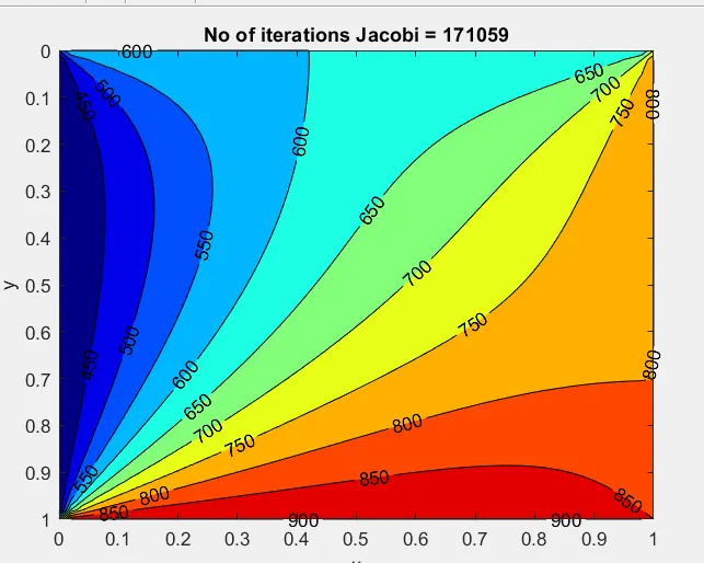
1) Jacaobi method:
2)Gauss-siedal method
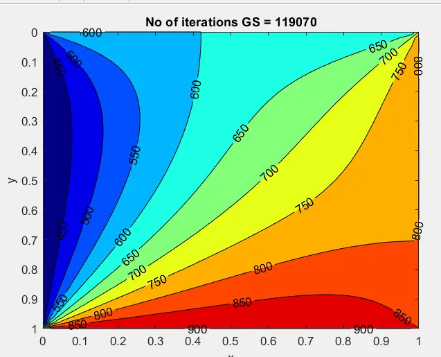
3)Successive overelaxation (SOR)
From above figures we can observe that when the solution converges, the number of iterations required for Jacobi method are very high as compared to Gauss-siedal method and SOR method.
B. Unsteady state 2D heat conduction
2D unsteady state heat conduction is given as,
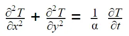
Solving above equation by numerical discretization,we get
I. Explicitily solving

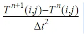
Here n denotes time step and i,j denotes space point at which temperature is to be evaluated
Solving for T(i,j) explicitly we get ,

K1=(alpha*dt)/(dx)^2;
K2=(alpha*dt)/(dy)^2;
II. Implicit solving

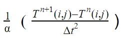
Solving for T(i,j) we get;

where,
K1=(alpha*dt)/(dx^2)
K2=(alpha*dt)/(dy^2)
Matlab code for explicit and implicit scheme for 2d unsteady state heat conduction ;
clear all
close all
clc


%given boundary condition
T_top=600;
T_bottom=900;
T_left=400;
T_right=800;
alpha=1.8;

%defining grid points
nx=10;
x=linspace(0,1,nx);
dx=x(2)-x(1);
ny=nx;
y=linspace(0,1,ny);
dy=y(2)-y(1);


T=300*ones(nx,ny);
T(:,end)=T_right;                      %temp at right
T(:,1)=T_left;                         %temp at right
T(1,:)=T_top;                          %temp at top
T(end,:)=T_bottom;                     %temp at bottom

%CORNER TEMPERATURES
T(end,end)=(T_bottom+T_right)/2;
T(1,end)=(T_top+T_right)/2;
T(1,1)=(T_top+T_left)/2;
T(end,1)=(T_bottom+T_left)/2;


%defining grid points
nx=10;
x=linspace(0,1,nx);
dx=x(2)-x(1);
ny=nx;
y=linspace(0,1,ny);
dy=y(2)-y(1);


dt=0.001;
t=100;
nt=t/dt;

error=9e9;
tol=1e-4;


K1=(alpha*dt)/(dx)^2;
K2=(alpha*dt)/(dy)^2;
T_old=T;


for k=1:nt
        iteration=0;
        while(error>tol)
        for i=2:nx-1
            for j=2:ny-1

                T(i,j)=T_old(i,j)*(1-2*K1-2*K2)+K1*(T_old(i+1,j)+T_old(i-1,j))+
                           K2*(T_old(i,j+1)+T_old(i,j-1));

            end
        end

        error=max(max(abs(T-T_old)));
        T_old=T;
        iteration=iteration+1;
    end
end
figure(1)
C = contourf(x,y,T,'ShowText','on');
xlabel('x')
ylabel('y')
set(gca,'YDIR','reverse')
colormap(jet)
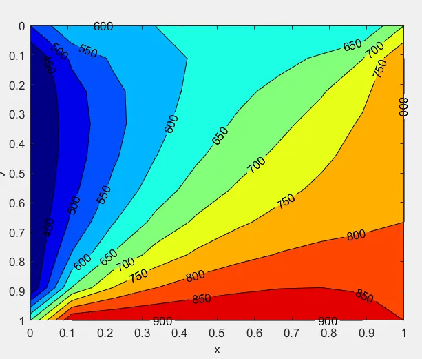
Explicit results:
Matlab code for implicit scheme:
clear all
close all
clc

%given boundary condition
T_top=600;
T_bottom=900;
T_left=400;
T_right=800;
alpha=1.8;

%defining grid points
nx=50;
x=linspace(0,1,nx);
dx=x(2)-x(1);
ny=nx;
y=linspace(0,1,ny);
dy=y(2)-y(1);


T=300*ones(nx,ny);
T(:,end)=T_right;                      %temp at right
T(:,1)=T_left;                         %temp at right
T(1,:)=T_top;                          %temp at top
T(end,:)=T_bottom;                     %temp at bottom

%CORNER TEMPERATURES
T(end,end)=(T_bottom+T_right)/2;
T(1,end)=(T_top+T_right)/2;
T(1,1)=(T_top+T_left)/2;
T(end,1)=(T_bottom+T_left)/2;


%defining time step
dt=0.001;
t=100;
nt=t/dt;

error=9e9;
tol=1e-4;

T_old=T;
T_prev=T;

K1=(alpha*dt)/(dx^2);
K2=(alpha*dt)/(dy^2);

iterative_solver=1

if iterative_solver==1  %Jacobi_method
    Jacobi_iter=0;
    for k=1:nt

    while(error>tol)

       for i=2:nx-1
          for j=2:ny-1
                    T(i,j)=(T_old(i,j)+K1*(T_old(i+1,j)+T_old(i-1,j))+K2*(T_old(i,j+1)+T_old(i,j-1)))/(1+2*K1+2*K2);
          end
       end
            error=max(max(abs(T_old-T)));
            T_old=T;
            Jacobi_iter=Jacobi_iter+1;
        end

        T_prev=T;
    end
    figure(1)
    [C,h]= contourf(x,y,T,'ShowText','on');
    xlabel('x')
    ylabel('y')
    set(gca,'YDIR','reverse')
    colorbar
    colormap(jet)
    clabel(C,h)
    title_text=sprintf('No of iterations Jacobi = %d',Jacobi_iter);
    title(title_text)
end


if iterative_solver==2         %Gauss_siedal
    Gauss_siedal_iter=0;
    for k=1:nt

    while(error>tol)

       for i=2:nx-1
          for j=2:ny-1
                    T(i,j)=(T_old(i,j)+K1*(T_old(i+1,j)+T(i-1,j))+K2*(T_old(i,j+1)+T(i,j-1)))/(1+2*K1+2*K2);
          end
       end
            error=max(max(abs(T_old-T)));
            T_old=T;
            Gauss_siedal_iter=Gauss_siedal_iter+1;
        end

        T_prev=T;
    end
    figure(2)
    [C,h]= contourf(x,y,T,'ShowText','on');
    xlabel('x')
    ylabel('y')
    set(gca,'YDIR','reverse')
    colorbar
    colormap(jet)
    clabel(C,h)
    title_text=sprintf('No of iterations Gauss_siedal_iter = %d',Gauss_siedal_iter);
    title(title_text)
end


if iterative_solver==3  %SOR
    SOR_iter=0;
    beta=1.8;
    for k=1:nt

    while(error>tol)

       for i=2:nx-1
          for j=2:ny-1
                    T(i,j)=(T_old(i,j)+K1*(T_old(i+1,j)+T(i-1,j))+K2*(T_old(i,j+1)+T(i,j-1)))/(1+2*K1+2*K2);
                    T(i,j)=T_old(i,j)*(1-beta)+(beta*T(i,j));
          end
       end
            error=max(max(abs(T_old-T)));
            T_old=T;
            SOR_iter=SOR_iter+1;
        end

        T_prev=T;
    end
    figure(3)
    [C,h]= contourf(x,y,T,'ShowText','on');
    xlabel('x')
    ylabel('y')
    set(gca,'YDIR','reverse')
    colorbar
    colormap(jet)
    clabel(C,h)
    title_text=sprintf('No of iterations SOR = %d',SOR_iter);
    title(title_text)
end
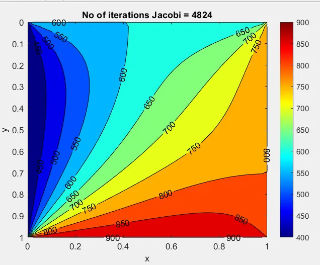
1. Jacobi method:
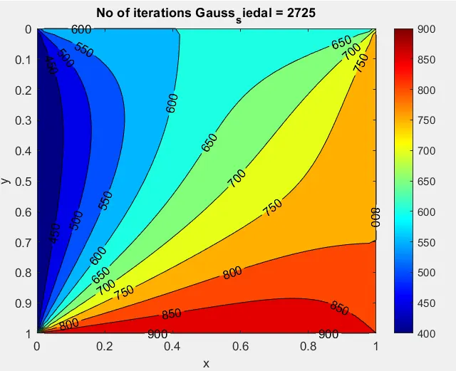
2. Gauss-siedal method
3. Successive over realxation (SOR)
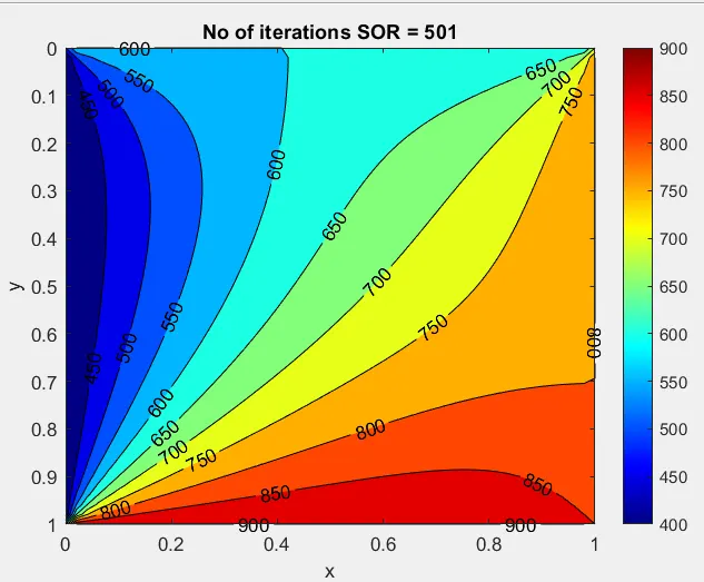
Here the number of iterations for jacobi are much higher than Gauss-siedal and SOR.