Week 5 - Rayleigh Taylor Instability

AIM:

Simulate the Rayleigh Taylor Instability using ANSYS Fluent.

Expected results:

• What are some practical CFD models that have been based on the mathematical analysis of Rayleigh Taylor waves? In your own words, explain how these mathematical models have been adapted for CFD calculations.
• Perform the Rayleigh Taylor instability simulation for 2 different mesh sizes with the base mesh being 0.5 mm.
• Compare the results by showing the animations (Convert Video to GIF). Observe the differences in the animation and explain the effect of mesh size on simulation. Also, explain why a steady-state approach might not be suitable for these types of simulation. [Choose Air and Water for this simulation]
• Run one more simulation with water and user-defined material (density = 400 kg/m³, viscosity = 0.001 kg/m-s) for refined mesh.
• Define the Atwood Number. Find out the Atwood number for both the cases and explain how the variation in Atwood number in the above two cases affects the behavior of the instability.

INTRODUCTION:

The Rayleigh-Taylor instability is a fingering instability of an interface between two fluids of different densities, which occurs when the heavier fluid pushes the lighter fluid upward, creating large vortices and chaotic mixing. This phenomenon has applications in various engineering fields, such as combustion, astrophysics, and inertial confinement fusion.

Computational Fluid Dynamics (CFD) models have been developed to predict the RTI's behavior accurately and provide insight into the underlying physics.

One of the most common Computational Fluid Dynamics models for Rayleigh Taylor Instability is based on the Navier-Stokes equations, which are the fundamental equations governing fluid flow. To solve these equations, numerical methods such as finite element, finite volume, or finite difference methods are employed.

Another commonly used model for Rayleigh Taylor Instability is the Volume of Fluid (VOF) method. This method is particularly well-suited for problems with a sharp interface between two fluids. In VOF, the fluid interface is explicitly tracked, and the governing equations are solved for each fluid phase separately. The interface is then reconstructed based on the volume fractions of each fluid, which are determined by solving a transport equation for the interface.

In addition to these models, there are also lattice Boltzmann methods, which are based on the Boltzmann equation for particle distribution functions. These models can accurately simulate complex fluid phenomena, such as multiphase flow, and are becoming increasingly popular in RTI simulations.

Overall, CFD models have been adapted to accurately predict the behavior of RTI by solving the Navier-Stokes equations, explicitly tracking the fluid interface with the VOF method, or using the lattice Boltzmann method. These models have been used in various applications, such as predicting mixing in inertial confinement fusion, and understanding the behavior of supernova explosions.

By applying these mathematical models and adapting them for CFD calculations, researchers and engineers can gain insights into the behavior of Rayleigh-Taylor waves. These simulations enable the prediction of quantities of interest such as interface evolution, mixing rates, and energy transfer, which are crucial for understanding and designing systems involving RT waves, such as inertial confinement fusion, supernovae explosions, and various engineering applications involving multiphase flows.

THEORY:

Multiphase Flow:

Multiphase flow is a simulatneous flow of materials with different states or phases such as liquid and gas. It is a flow of materials with different chemical properties but in same state or phase such as liquid and liquid.

Volume of Fluid Method:

Volume of fluid method is a surface tracking method. It is designed to find out the position of interface between the two or more immiscible fluids. The volume fraction of each fluid in each of the cell through out domain can be tracked by usinhg this method. In this method, all the control volumes must be filled with single phase or combination of phases. The summation of the two phases for VOF should be equal to 1.

Courant Number:

Courant Number is a non-dimensional number which is the ratio of the numerical time step size to the characteristic time scale of the problem multiplied by the characteristic wave speed. Courant number is often limited to a value of 1.

Atwood Number:

The Atwood number is a dimensionless parameter that is commonly used in fluid mechanics to characterize the instability of two fluids with different densities when they are brought into contact. It is defined as the difference between the densities of the two fluids divided by their sum, i.e.,

At = (ρ₁ - ρ₂) / (ρ₁ + ρ₂)

where ρ₁ and ρ₂ are the densities of the two fluids, At is the Atwood number.

SOLVING & MODELING APPROACH:

In this simulation, two fluids i.e. air and water, flows simultaneously in a rectangular geometry using laminar model and transient time state until the denser fluid reaches the bottom and pushes the lighter fluid upward i.e. water pushes the air upward as the density of water is greater than that of air using coarse and refined mesh. Another simulation will be done between an User-defined material whose density = 400 Kg/m³, viscosity = 0.001 kg/m-s and water by using refined mesh.

PRE-PROCESSING AND SOLVER SETTING:

Geometry:

• Run ANSYS 2023 R1 student version and drag Fluid Flow (Fluent) in the project Schematic and then run ANSYS Space Claim by selecting it from Geometry.
• Create a rectangle from the origin by using the Rectangle tool.
• Convert the rectangle to 3D surface by using the Pull tool.
• Create another component below the previous surface from the origin and convert it into a 3D surface.

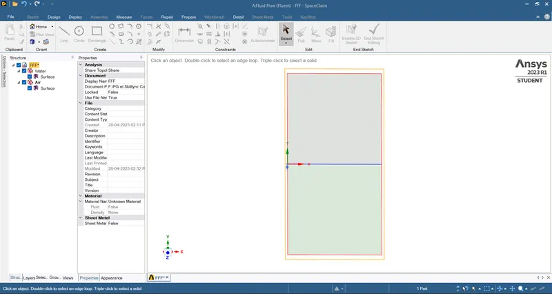
• Share the topology by using the share tool, to share the interface between both the surface.

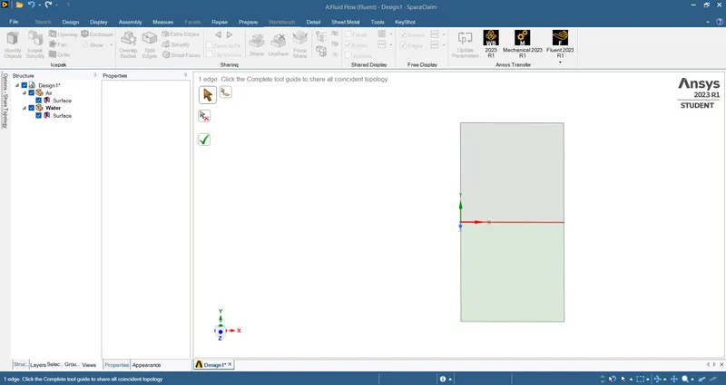
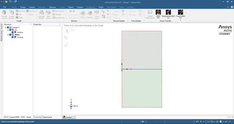
Mesh:

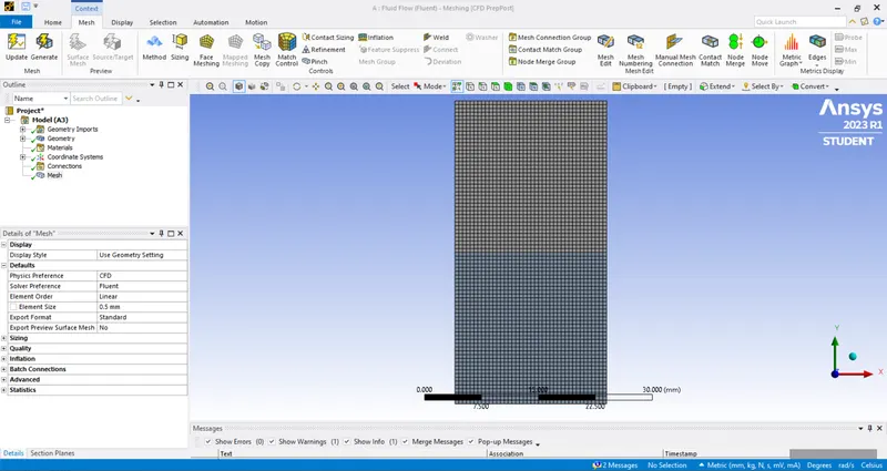
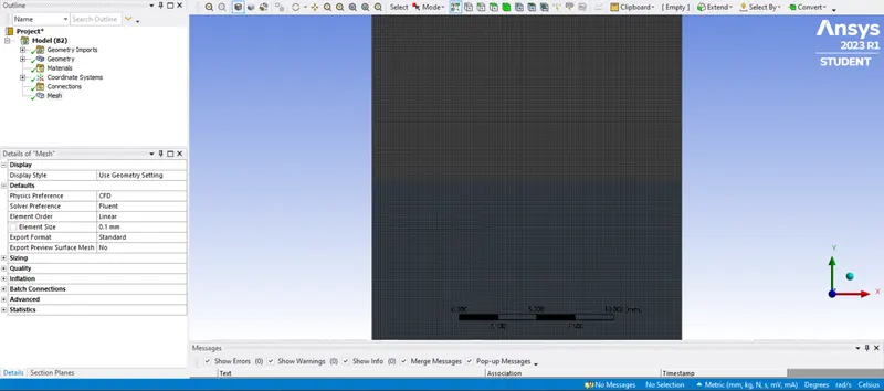
• Create a base mesh with element size of 0.5 mm for the 1st simulation and a refined mesh of 0.1 mm for the 2nd and 3rd simulations.
• Mesh with element size of 0.5 mm is shown below:

• Refined Mesh with element size of 0.1 mm is shown below:

Setup:

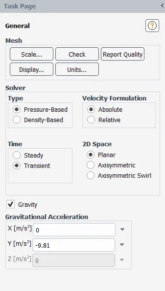
• Under general settings, select pressure-Based type solver, Transient time, Gravity and assign Gravitational acceleration as -9.81 m/s² in the Y-axis.

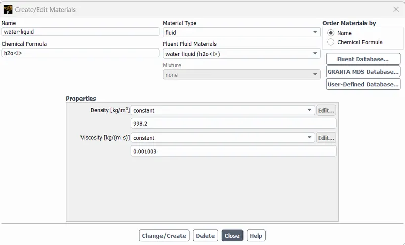
• Select water and air as fluids in the material selection section.

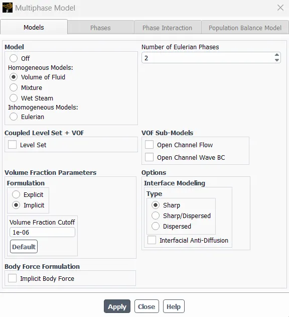
• Select Volume of fluid and implicit formulation under Multiphase model section and click apply.

• Under Multiphase Model phases section rename the primary phase as air and secondary phase as water and click apply.

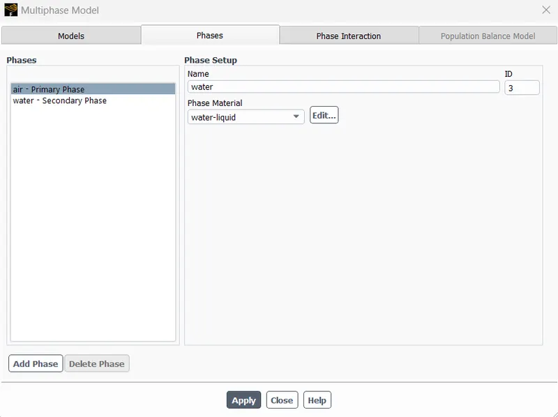
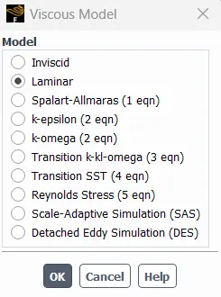
• Select Laminar under Viscous model.

• Initialize the solution by selecting Standard initialization and coupled method.
• Create contour for volume fraction of water.

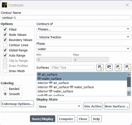
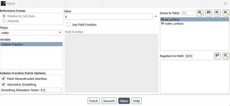
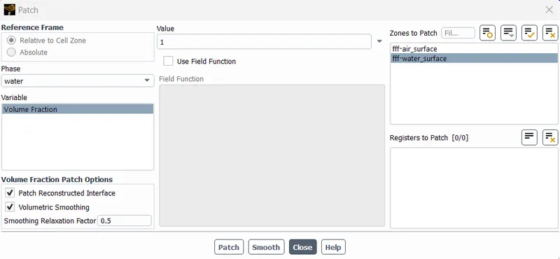
• Select Patch option and selecting water as phase assign the value of volume fraction of air as 0 and click patch, and water as 1 and again patch it.

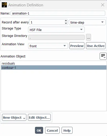
• Create solution animation by selecting the appropriate contour to capture the flow and mixing between the interfaces.

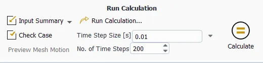
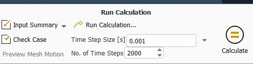
• Assign Time step size as 0.01 and No. of time steps until the proper solution has been achieved for the 1st simulation. Assign time step size as 0.001 for the 2nd simulation and 0.005 for the 3rd simulation. Run calculate after assigning the datas.

RESULTS:

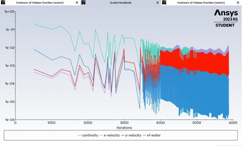
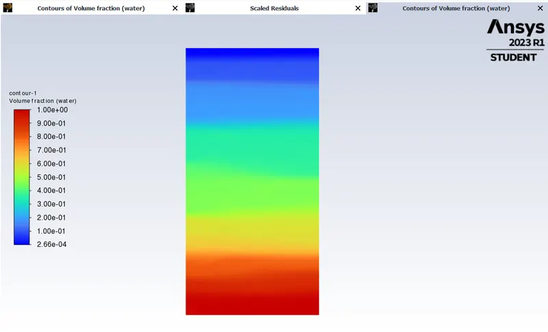
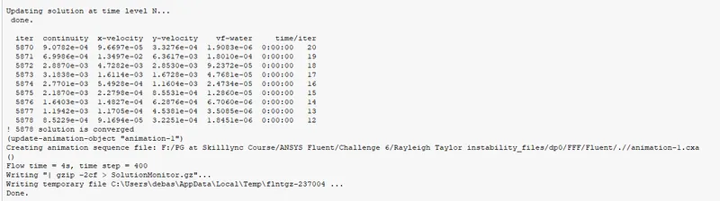
• 1st simulation taking mesh size as 0.5 mm, time step size as 0.01 and No. of Time steps done as 400 resulting in total flow time as 4 seconds.

Scaled Residuals:

Contour of Volume fraction:

Total flow time and time step:

Solution animation:

Animation file: https://drive.google.com/file/d/1mhSmCsfs7H90l_dUvWkSPkB2ghUT6JtI/view?usp=share_link

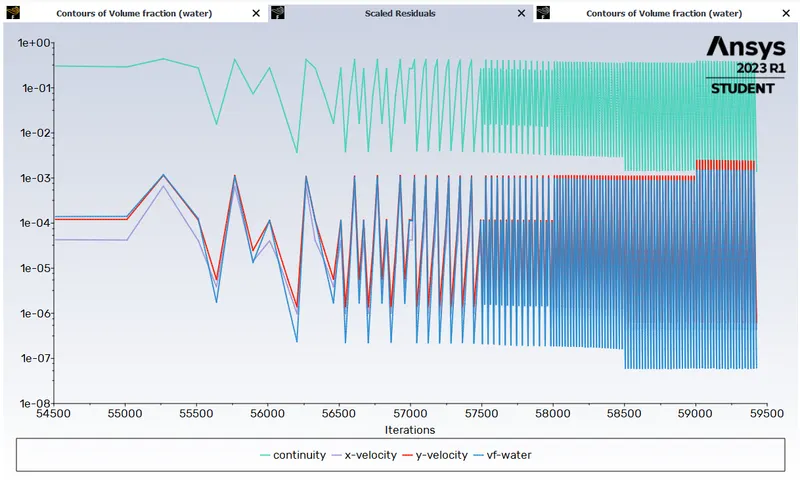
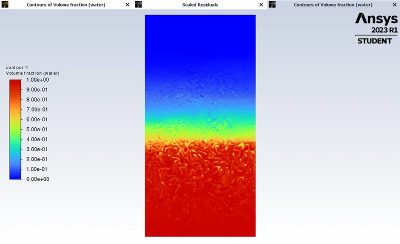
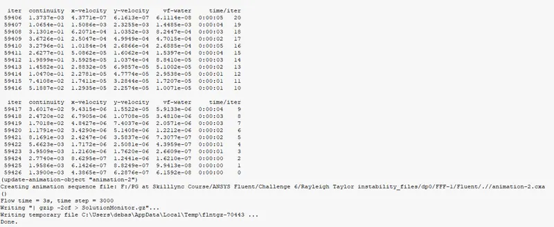
• 2nd simulation taking mesh size as 0.1 mm, time step size as 0.001 and No. of Time steps done as 3000 resulting in total flow time as 3 seconds.

Scaled Residuals:

Contour of Volume fraction:

Total flow time and time step:

Solution animation:

Animation file: https://drive.google.com/file/d/1uVc61m7k7DpdQLHy7XURIHIZNNW2qplK/view?usp=share_link

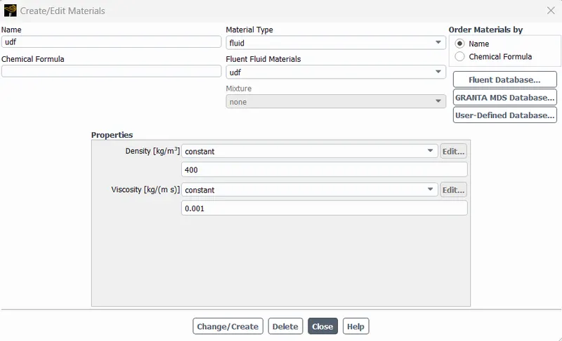
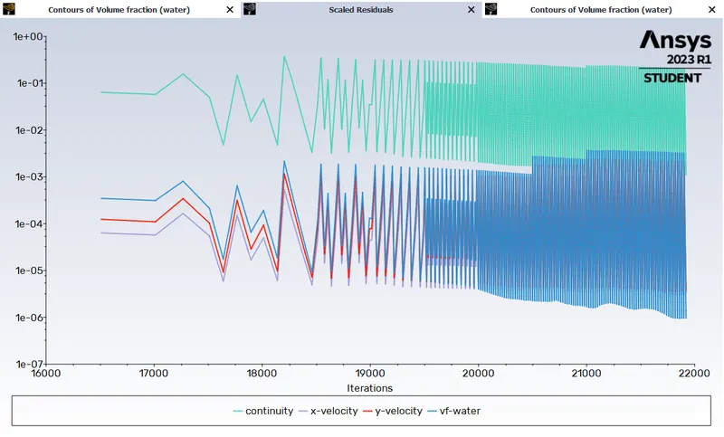
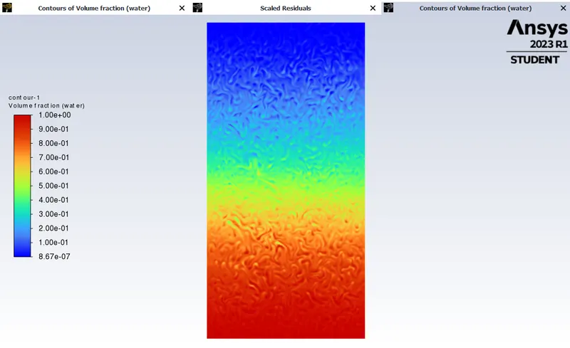
• 3rd simulation taking mesh size as 0.1 mm, time step size as 0.005 and No. of Time steps done as 1100 resulting in total flow time as 5.5 seconds.

Properties for User Defined Material:

Scaled Residuals:

Contour of Volume fraction:

Total flow time and time step:

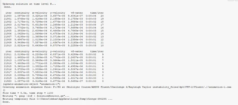
CONCLUSIONS:

• Comparing the animations between the 1st and 2nd simulations, where the mesh size for 1st simulation is 0.5 mm and 0.1 mm for the 2nd simulation, it is seen that the animation with more refined mesh has better resolution in the interfacial region between the two fluids. The animation with mesh size as 0.5 mm couldn't capture the small- scale structures and turbulence, which can be properly seen in the simulation with more refined mesh. The drawback of using more refined mesh leads to more computational time, but it gives much better predictions of mixing and evolution of instability.
• The steady-state approach is not suitable for simulating Rayleigh-Taylor instability (RTI) because RTI is an inherently unsteady phenomenon that involves the growth and evolution of instabilities over time. In a steady-state simulation, the flow is assumed to be time-invariant, and the solution is assumed to have reached a stable equilibrium state. RTI involves the growth and evolution of unstable interfaces over time. Therefore a transient state approach is suitable.
• For the 3rd simulation where the viscosity of the udf is higher than that of air has more growth and evolution of instabilities in the interfacial region.
• The Atwood number between air & water is -0.99.76.. and the Atwood number between UDF & water is -0.429. It is seen that the Atwood number between air & water is relatively small resulting in weaker bouyancy forces and slow evolution, with small scale mixing patterns and well-defined interfaces between the two fluids where between the UDF & water the mixing of the two fluids is very violent as the densities of both the fluids is higher which increases the instability due to which evolution is more rapid, resulting in large scale mixing patterns and less well- defined interfaces between the two fluids.
• Therefore, as Atwood number increases, the Rayleigh-Taylor Instability becomes more violent and mixing between the two fluids becomes more complex and unpredictable.