Week 5 - Rayleigh Taylor Instability

Objectives

1. What are some practical CFD models that have been based on the mathematical analysis of Rayleigh Taylor waves? In your own words, explain how these mathematical models have been adapted for CFD calculations.
2. Perform the Rayleigh Taylor instability simulation for 2 different mesh sizes with the base mesh being 0.5 mm. Compare the results by showing the animations( Attach them from your google drive). Observe the differences in the animation and explain the effect of mesh size on the simulation. Also, explain why a steady-state approach might not be suitable for these types of simulations.[ Choose Air and Water for this simulation]
3. Run one more simulation for refined mesh with water and user-defined material(density = 400 kg/m³, viscosity = 0.001 kg/m-s).
4. Define the Atwood Number. Find out the Atwood number for both cases and explain how the variation in the Atwood number in the above two cases affects the behaviour of the instability.

Rayleigh Taylor Instability

The Rayleigh–Taylor instability, or RT instability, is an instability of an interface between two fluids of different densities which occurs when the lighter fluid is pushing the heavier fluid. Examples include the behaviour of water suspended above oil in the gravity of Earth, mushroom clouds like those from volcanic eruptions and atmospheric nuclear explosions, supernova explosions in which expanding core gas is accelerated into denser shell gas, stabilities in plasma fusion reactors and inertial confinement fusion. It is clear from Newton's law of viscosity, fluid cannot resist the slightest shear force and Density is one of the main properties of the fluid to incorporate the shear force. Based on the density, when lighter and heavier fluids are mixed, denser fluid comes to top of the lighter fluid, due to gravity and the density variation at the interface of the liquid is not stable.

Some practical CFD models that have been based on the mathematical analysis of Rayleigh Taylor waves

1. The Richtmyer–Meshkov instability (RMI) occurs when two fluids of different densities are impulsively accelerated. Normally this is by the passage of a shock wave. The development of the instability begins with small amplitude perturbations which initially grow linearly with time. This is followed by a nonlinear regime with bubbles appearing in the case of a light fluid penetrating a heavy fluid, and with spikes occurring in the case of a heavy fluid penetrating a light fluid. A chaotic regime eventually is reached and the two fluids mix. This instability can be considered the impulsive-acceleration limit of the Rayleigh Taylor instability.
2. The Kelvin–Helmholtz instability is a fluid instability that occurs when there is velocity shear in a single continuous fluid or a velocity difference across the interface between two fluids. Kelvin-Helmholtz's instabilities are visible in the atmospheres of planets and moons, such as in cloud formations on Earth or the Red Spot on Jupiter, and the atmospheres of the Sun and other stars.
3. The Plateau–Rayleigh instability, often just called the Rayleigh instability, explains why and how a falling stream of fluid breaks up into smaller packets with the same volume but less surface area. It is related to the Rayleigh–Taylor instability and is part of a more excellent branch of fluid dynamics concerned with fluid thread breakup

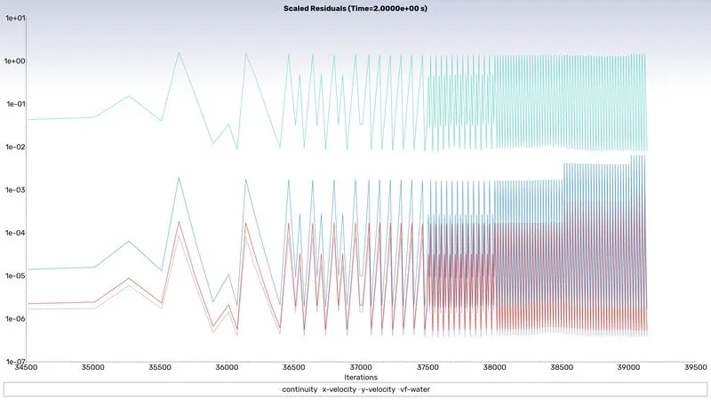
Here we used time-based solving to chive the result so we need to consider the proper time step value to maintain the solution or the solution travels more than the cell distance leading to solution acceleration and throwing a floating point exception error.

Floating point exception error

A floating point exception is an error that occurs when you try to do something impossible with a floating point number, such as dividing by zero. In fluent floating point error can be caused by many factors such as improper mesh size, and defining some properties close to zero.

STEPS TO BE FOLLOWED

In this process, three cases have been used to study Rayleigh Taylor's Instability.

Case 1:water and air have working fluid with 0.5 mm mesh.

Case 2:water and air have working fluid with 0.1 mm mesh.

Case 2:water and UDM(Density=400 kg/m3,viscosity=0.001kg/ms) have working fluid with 0.1 mm mesh.

Step 1: Initially, start with creating the geometry in SpaceClaim and prepare it for a multi-phase flow analysis

1. Create a square of 20 mm*20 mm. Use the Pull tool to create a surface.
2. Move the generated component to the New Component. Name it Air.
3. Now click on design and create a new component --> Water.
4. Repeat the sketch just above the Air with similar dimensions as mentioned.
5. Workbench > click on Share > Ok.

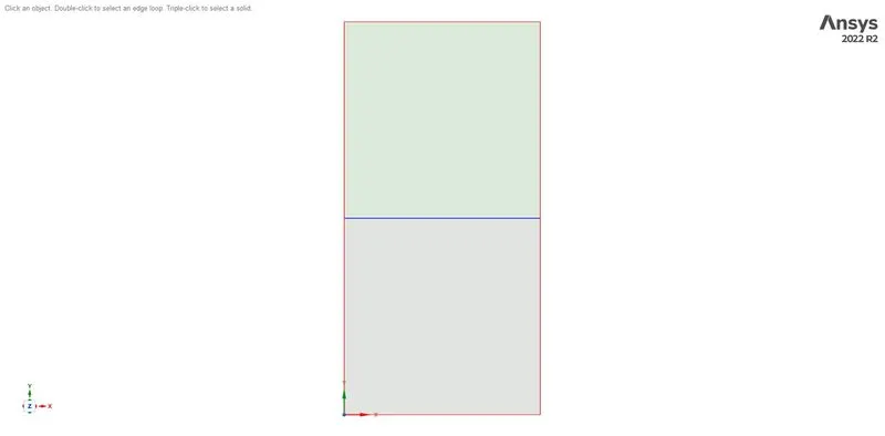
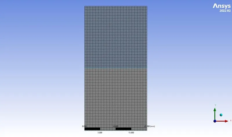
Step 2: From the created geometry mesh the surface with elements size of 0.5 mm for coarse mesh and 0.1mm for fine mesh.

Coarse mesh

Fine mesh

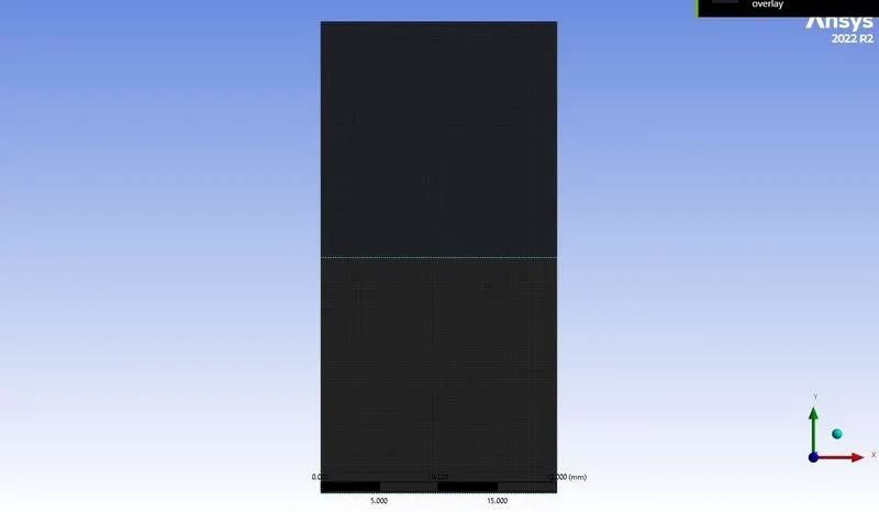
After generating the mesh, the number of nodes and elements is investigated using the statistics option. Then the mesh quality is checked by choosing the mesh matrices option in the quality section.

Step 3:In this step, the meshed geometric file has been imported to the fluent module and set the following conditions as follows in the fluent in solving the problem.

This procedure will be constant for the short tee and long tee with a momentum ratio

SOLVER TYPE	Pressure based
VELOCITY FORMULATION	Absolute
TIME	Transient state
VISCOUS MODEL	laminar
MATERIAL	Water Air user-defined material (UDM) `rho=400 (kg)/m^3` `mu=0.001 (kg)/(ms)`
Multiphase	Volume of fluid Number of eulerian phase=2 For case 1&2 it will be water and air For case 3 it will be water and udm
Initialization	Hybrid
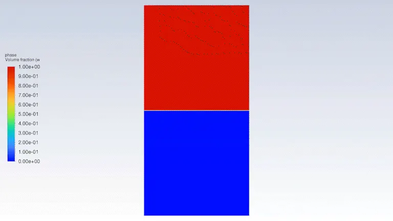
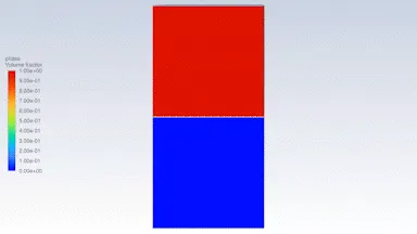
Patch	Patch water for the top region Patch air or UDM in the bottom region

the hybrid scheme is used for the initialization

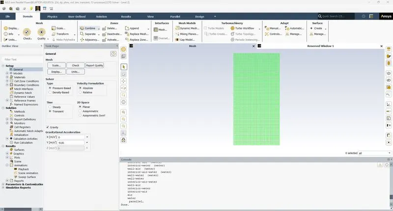
Patch

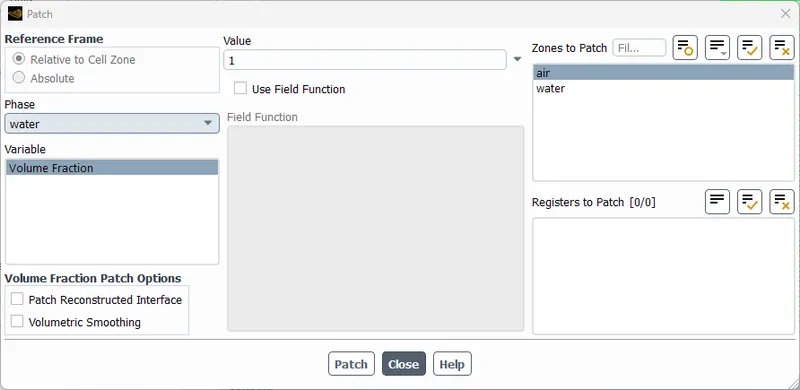
Phase contour after patch

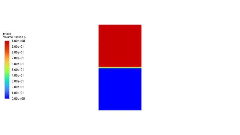
Results

Case 1

Residual plot

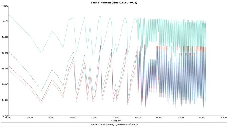
Phase contour

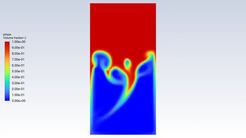
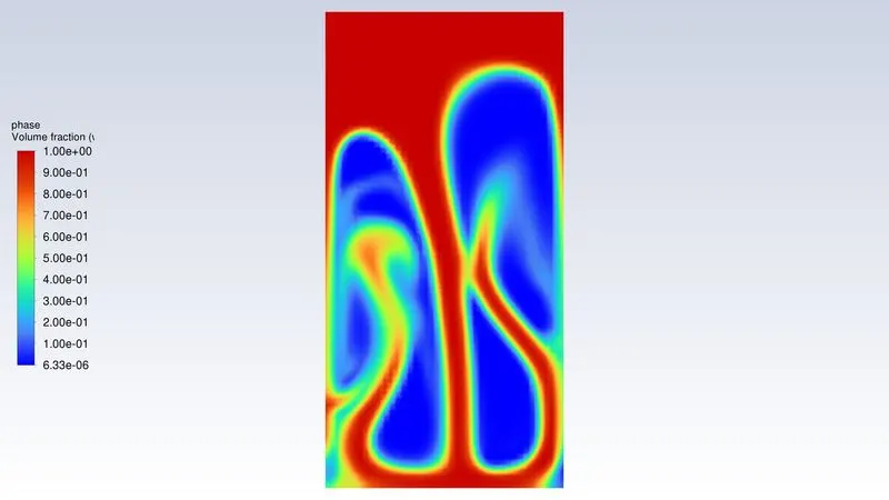
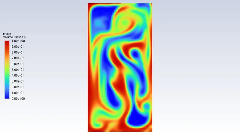
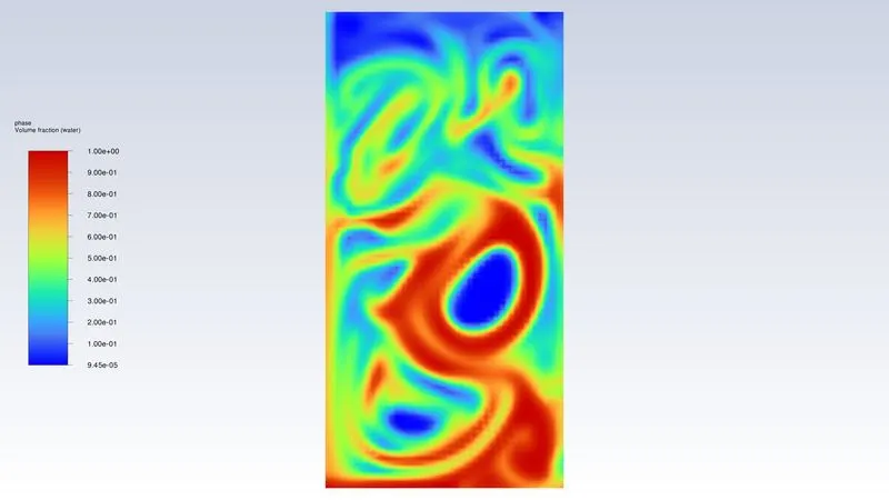
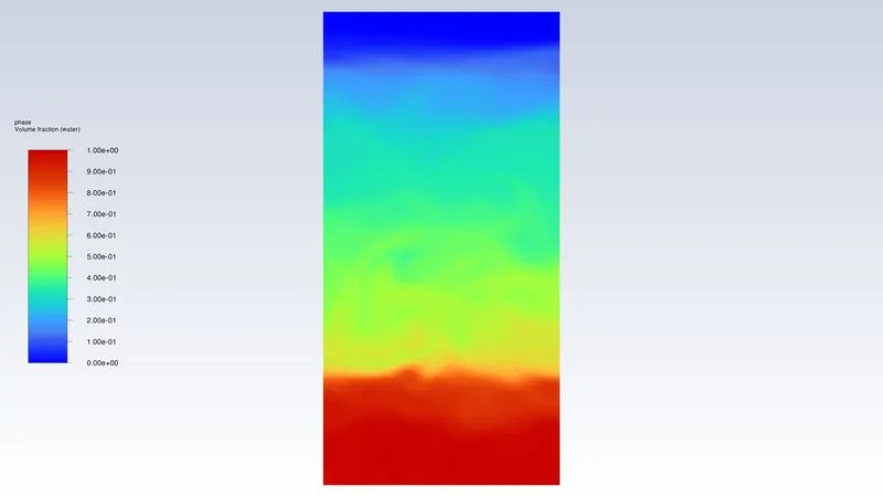
Animation

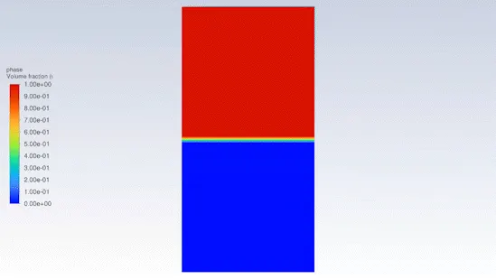
Case 2

Residual plot

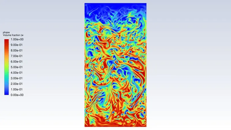
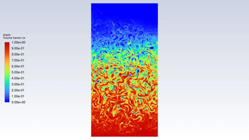
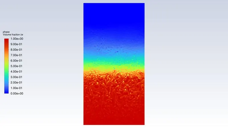
Phase contour

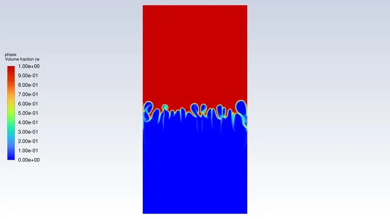
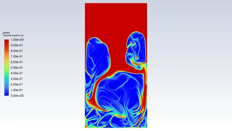
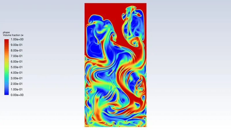
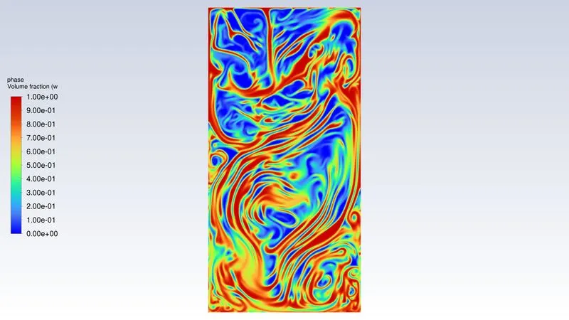
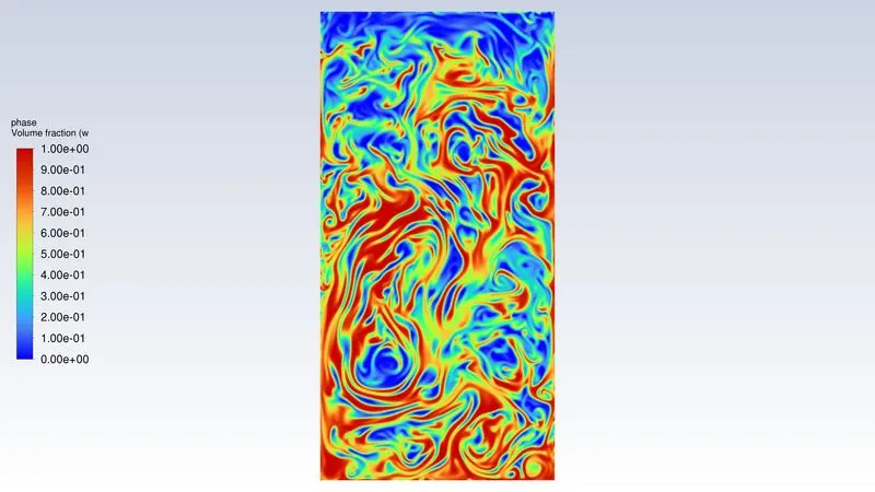
Animation

Case 3

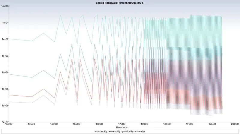
Residual plot

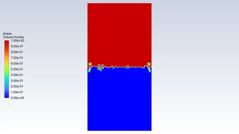
Phase contour

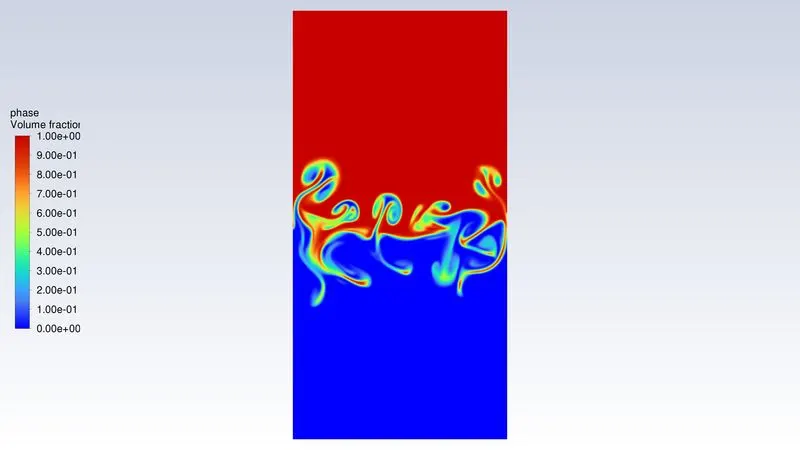
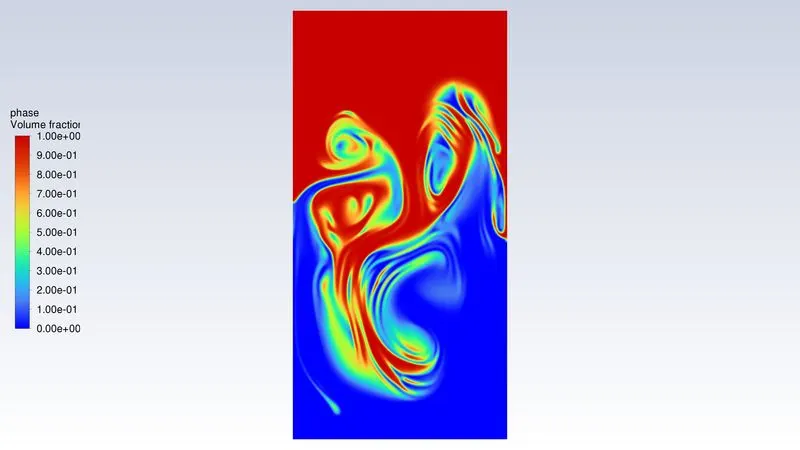
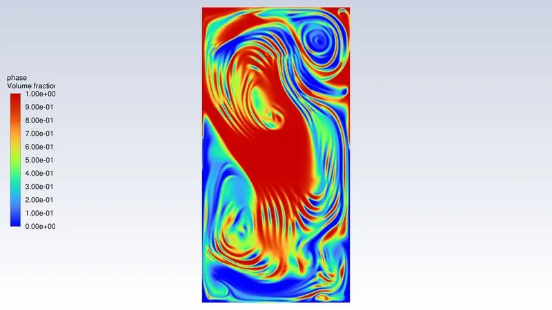
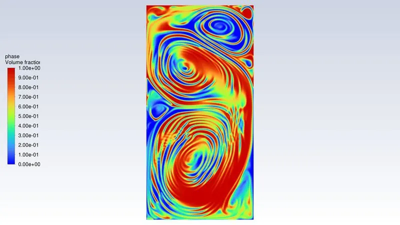
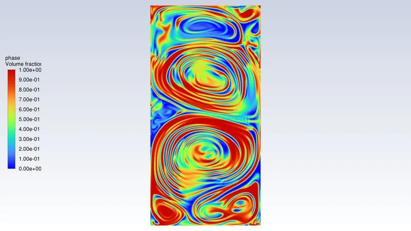
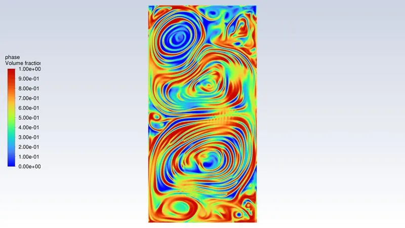
Animation

Solution discussion

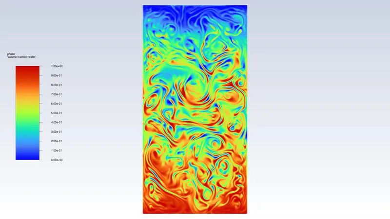
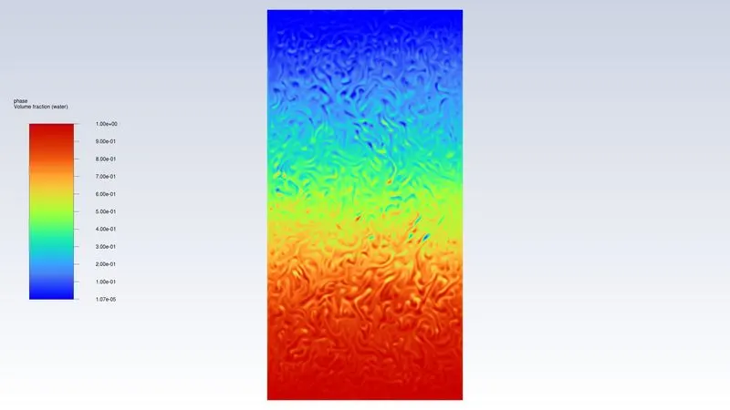
1. From the above cases, we observe that finer mesh captures the instability better than the coarse mesh, but it takes more computational time and we need to go minimum time step size to avoid floating point exception error.
2. From the contour lower-density fluid (Air) is settled on top and the higher-density fluid (bottom) is settled at the bottom due to the pushing of light fluid (air) instability forms due to gravity. These growing instabilities are known as Rayleigh Taylor Instability.
3. The Rayleigh Taylor instability forms in between the interfering region and lower-density fluid pushing a higher-density fluid due to shock waves occurring at the interface. This lead to the formation of a bubble and swirl and compresses the heavy fluid around it. Later disturbance at the interface ends with lighter fluid settling up and the heavier fluid settling down.

Atwood Number.

The Atwood number (A) is a dimensionless number in fluid dynamics used in the study of hydrodynamic instabilities in density-stratified flows. It is a dimensionless density ratio defined as

`A=(rho_1-rho_2)/(rho_1+rho_2)`

where

`rho`-density of the fluid

The Atwood number is an important parameter in the study of Rayleigh–Taylor instability and Richtmyer–Meshkov instability. In Rayleigh–Taylor instability, the penetration distance of heavy fluid bubbles into the lighter fluid is a function of the acceleration time scale, `A g t^2` where g is the gravitational acceleration and t is the time.

Atwood number close to 0, RT instability flows take the form of the asymmetric finger of fluid;

Atwood number close to 1, the much lighter fluid “below” the heavier fluid takes the form of a larger bubble.

CASE	PHASE	DENSITY OF PHASE 1 `rho_1`	DENSITY OF PHASE 2 `rho_2`	ATWOOD NUMBER
1&2	WATER & AIR	998.2	1.225	0.99754
3	WATER & uDM	998.2	400	0.42783