Week 5.1 - Mid term project - Solving the steady and unsteady 2D heat conduction problem

GIVEN

Solve the 2D heat conduction equation by using the point iterative techniques

Boundary conditions

Top Boundary = 600 K

Bottom Boundary = 900 K

Left Boundary = 400 K

Right Boundary = 800 K

Solve the problem using Steady state analysis & Transient State Analysis

You will implement the following methods for solving implicit equations

1. Jacobi

2. Gauss-seidel

3. Successive over-relaxation

Your absolute error criteria are 1e-4

2D heat conduction

The process by which heat is transferred from the hotter end to the colder end of the object is known as conduction. According to thermodynamic systems, heat transfer is defined as the movement of heat across the system's border due to a difference in temperature between the system and its surroundings.

In conduction, the heat flow is within and through the body itself.2D heat conduction is the conduction of heat calculation in two dimensions. Here we solve the steady and unsteady 2D heat conduction problem

Steady-state conduction

Steady-state conduction is the form of conduction that happens when the temperature difference(s) driving the conduction are constant, after an equilibration time. steady-state conduction, the amount of heat entering any region of an object is equal to the amount of heat coming out.

The formula for steady-state 2D heat conduction without heat generation is

`(del^2T)/(del x^2)+(del^2T)/(del y^2)=0`

By discretizing the above equation and spacing between the two discrete points in the x & y direction are dx and dy respectively. Now we try to formulate the problem in such a way that we can set it up as a computer program.

`(T_L-2T_P+T_R)/(delx^2)+(T_T-2T_P+T_B)/(dely^2)=0`

`(2T_P)/(delx^2)+(2T_P)/(dely^2)=(T_L+T_R)/(delx^2)+(T_T+T_B)/(dely^2)`

`T_P[2(delx^2+dely^2)/(delx^2dely^2)]`

`k=[2(delx^2+dely^2)/(delx^2dely^2)]`

`T_P=1/k[[(T_L+T_R)/(delx^2)]+[(T_T+T_B)/(dely^2)]]`

We assume that we have uniform grid spacing in our problem so dx=dy

Transient conduction

During any period in which temperatures change in time at any place within an object, the mode of thermal energy flow is termed transient conduction.

The formula for Transient state 2D heat conduction without heat generation is

`(del T)/(del t)=alpha[(del^2T)/(del x^2)+(del^2T)/(del y^2)]`

The second-order partial differential in the left of the equal sign can be approximated by the central difference quotient

The temperature item on the right of the equal sign can be approximated by the first-order time forward difference quotient.

`(T_P^(n+1)-T_P^n)/(delt)=[(T_L-2T_P+T_R)/(delx^2)+(T_T-2T_P+T_B)/(dely^2)]^(n or n+1)`

Time interval,

n is for explicit schemes

n+1 is for implicit schemes

The final equations we end up with before developing it into a computer program are as follows:

For the Explicit method,

`T_P^(n+1)=T_P^n+K1[T_L-2T_P+T_R]^n+K2[T_T-2T_P+T_B]^n`

For the Implicit method,

`T_P^(n+1)=1/(1+2K1+2K2)[T_P^n+K1[T_L+T_R]^(n+1)+K2[T_T+T_B]^n`

where

`K1=alpha(delt)/(delx);K2=alpha(delt)/(dely)`

with this equation the created program

Program

%%
close all
clear all %#ok<CLALL>
clc

%input for heat conduction calculation and boundary condition

tic

l = 1;
nx = 10;
ny = nx;
dx = l/(nx-1);
dy = l/(ny-1);


x = linspace(0,1,nx);
y = linspace(0,1,ny);
T = ones(nx,ny);

T(2:nx-1,2:ny-1) = 300;
T(end,:) = 600;
T(1,:) = 900;
T(:,1) = 400;
T(:,end) = 800;
T(1,1) = (T(1,2)+T(2,1))/2;
T(1,end) = (T(1,ny-1)+T(2,ny))/2;
T(end,1) = (T(nx-1,1)+T(nx,2))/2;
T(end,end) = (T(nx-1,ny)+T(nx,ny-1))/2;

T_initial = T;
T_old = T;
T_prev_dt=T;

[xx,yy] = meshgrid(x,y);
tol = 1e-4;
error = 9e9;
omega = 1.1;
iter=1;

%% Defining the calculation as steady state or transient state
state = input('Enter 1 for study state, 2 for transient state = ');

%% study state
if state == 1
    K = 2*((dx^2 + dy^2)/(dx^2*dy^2));
    Iterative_solver = input('Enter 1 for Jacobi, 2 for Gauss Siedel and 3 for SOR = ');

    %% jacobi iteration of study state
    if Iterative_solver == 1
        error=9e9;
        while(error > tol)
            for i = 2:nx-1
                for j = 2:ny-1
                    term1 = ((1/K)*((T_old(i-1,j)+T_old(i+1,j))/dx^2));
                    term2 = ((1/K)*((T_old(i,j-1)+T_old(i,j+1))/dy^2));
                    T(i,j) = term1 + term2;
                end
            end
            error = max(max(abs(T_old-T)));
            T_old = T;
            iter = iter + 1;

            [A,B] = contourf(xx,yy,T);
            colorbar;
            colormap(jet)
            clabel(A,B)
            %pause(0.03)
            title(sprintf('Steady State Heat conduction using Jacobi method n Number of iterations: %d',iter))
        end
    end

    %% Gauss Siedel iteration of study state
    if Iterative_solver == 2
        error=9e9;
        while(error > tol)
            for i = 2:nx-1
                for j = 2:ny-1
                    term1 = ((1/K)*((T(i-1,j)+T_old(i+1,j))/dx^2));
                    term2 = ((1/K)*((T(i,j-1)+T_old(i,j+1))/dy^2));
                    T(i,j) = term1 + term2;
                end
            end
            error = max(max(abs(T_old-T)));
            T_old = T;
            iter = iter + 1;

            [A,B] = contourf(xx,yy,T);
            colorbar;
            colormap(jet)
            clabel(A.B)
            %pause(0.03)
            title(sprintf('Steady State Heat conduction using Gauss siedel method n Number of iterations: %d',iter))
        end
    end

    %% sor iteration of study state
    if Iterative_solver == 3
        iter = 1;
        error=9e9;
        while(error > tol)
            for i = 2:nx-1
                for j = 2:ny-1
                    term1 = ((1/K)*((T(i-1,j)+T_old(i+1,j))/dx^2));
                    term2 = ((1/K)*((T(i,j-1)+T_old(i,j+1))/dy^2));
                    T(i,j) = (1-omega)*T_old(i,j) + omega*(term1 + term2);
                end
            end
            error = max(max(abs(T_old-T)));
            T_old = T;
            iter = iter + 1;

            [A,B] = contourf(xx,yy,T);
            colorbar;
            colormap(jet)
            clabel(A,B)
            %pause(0.03)
            title(sprintf('Steady State Heat conduction using SOR method n Number of iterations: %d',iter))
        end
    end
end

%% Transient state
if state == 2
    alpha=1.4;
    t= input('time t = ');
    % here dx=dy take cfl no = 2.4
    cfl=0.21;
    dt=(cfl*(dx^2))/alpha;
    nt = round(t/dt);
    k1=(alpha*dt)/(dx^2);
    k2=(alpha*dt)/(dy^2);

    Method = input('Enter 1 for explicit, 2 for implicit = ');

    %% explicit method
    if Method == 1
        for time_step=1:nt
            error=9e9;
            while(error>tol)
                for i=2:nx-1
                    for j=2:ny-1
                        term1=T_old(i-1,j)-(2*T_old(i,j))+T_old(i+1,j);
                        term2=T_old(i,j-1)-(2*T_old(i,j))+T_old(i,j+1);
                        T(i,j)=T_old(i,j)+k1*term1+k2*term2;
                    end
                end
                error=max(max(abs(T_old-T)));
                T_old=T;
                iter=iter+1;
            end
        end
        figure(1)
        [A,B]=contourf(xx,yy,T);
        colorbar
        colormap(jet)
        clabel(A,B);
        title(sprintf('Unsteady state Explicit Iterations = %d',iter))
        %pause(0.03)
    end

    %% Implicit method
    if Method == 2

        Iterative_solver = input('Enter 1 for Jacobi, 2 for Gauss Siedel and 3 for SOR = ');
        %% time step
        for time_step = 1:nt
            if Iterative_solver==1
                Text=sprintf('Jacobie Iteration');
                term1=(1+2*k1+2*k2)^(-1);
                term2=k1*term1;
                term3=k2*term1;

                error=9e9;
                while(error>tol)
                    for i=2:nx-1
                        for j=2:ny-1

                            H=(T_old(i-1,j)+T_old(i+1,j));
                            V=(T_old(i,j-1)+T_old(i,j+1));
                            T(i,j) = (T_prev_dt(i,j)*term1)+(H*term2)+(V*term3);
                        end
                    end
                    error=max(max(abs(T_old-T)));
                    T_old=T;
                    iter=iter+1;
                end
            end

            if Iterative_solver==2
                Text=sprintf('Gauss Siedel Iteration');
                term1=(1+2*k1+2*k2)^(-1);
                term2=k1*term1;
                term3=k2*term1;

                error=9e9;
                while(error>tol)
                    for i=2:nx-1
                        for j=2:ny-1

                            H=(T(i-1,j)+T_old(i+1,j));
                            V=(T(i,j-1)+T_old(i,j+1));
                            T(i,j) = (T_prev_dt(i,j)*term1)+(H*term2)+(V*term3);
                        end
                    end

                    error=max(max(abs(T_old-T)));
                    T_old=T;
                    iter=iter+1;
                end
            end

            if Iterative_solver==3
                Text=sprintf('sor Iteration');
                term1=(1+2*k1+2*k2)^(-1);
                term2=k1*term1;
                term3=k2*term1;

                error=9e9;
                while(error>tol)
                    for i=2:nx-1
                        for j=2:ny-1

                            H=(T(i-1,j)+T_old(i+1,j));
                            V=(T(i,j-1)+T_old(i,j+1));
                            T(i,j) = (1-omega)*T_old(i,j)+omega*((T_prev_dt(i,j)*term1)+(H*term2)+(V*term3));
                        end
                    end

                    error=max(max(abs(T_old-T)));
                    T_old=T;
                    iter=iter+1;
                end
            end
            T_prev_dt=T;


        end
        figure(1)
        [A,B]=contourf(xx,yy,T);
        colorbar;
        colormap(jet);
        clabel(A,B);
        text=sprintf('Transient state Heat conduction using Implicit %s = %d\n',Text,iter);
        title(text)
        %pause(0.03)
    end
end
time=toc;

Output

2D heat conduction equation

contour get from the program

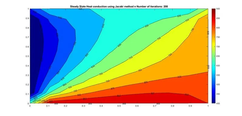
1. study-state Jacobi iteration

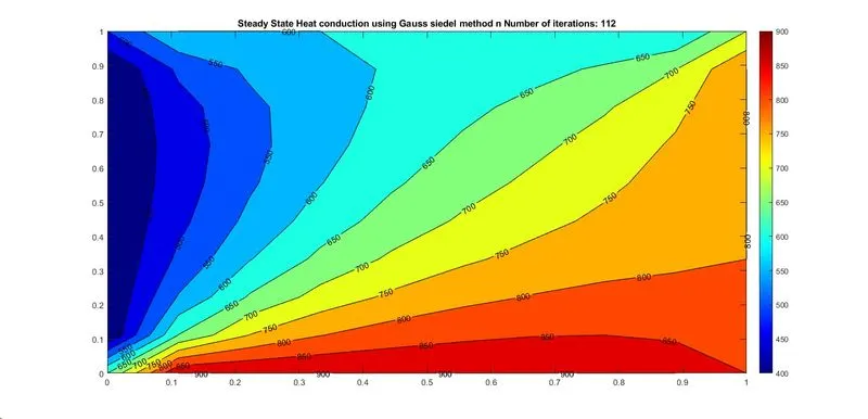
2.study-state Gauss-seidel iteration

3. study-state Successive over-relaxation iteration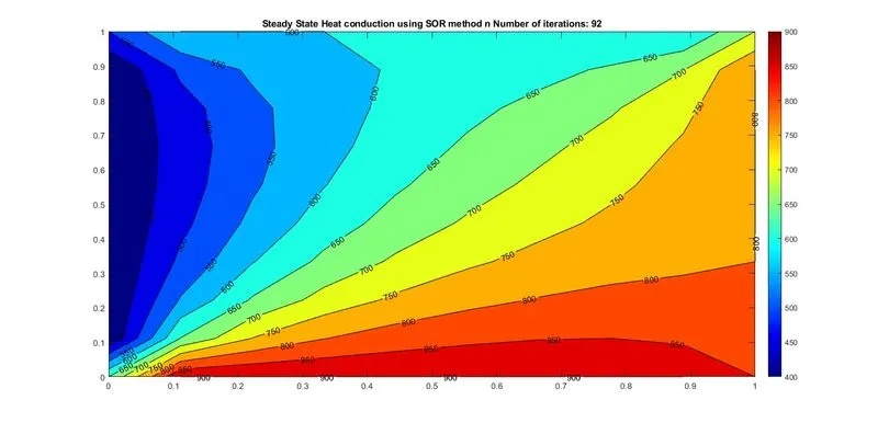

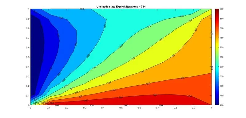
4. Transient State Explicit method

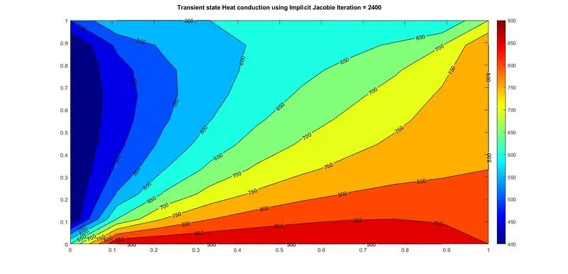
5. Transient State Implicit Jacobi iteration

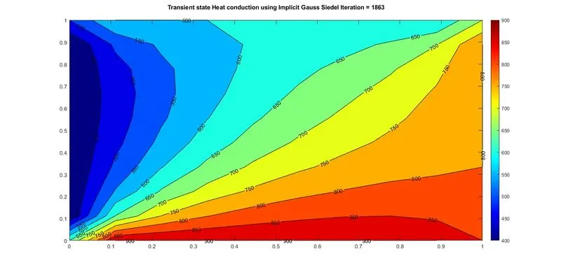
6. Transient State Implicit Gauss-seidel iteration

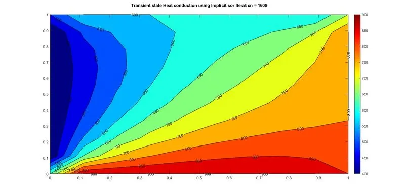
7. Transient State Implicit Successive over-relaxation iteration

Solution discussion

1. In steady-state methods, there is no time loop and the results converge within a few iterations. when we include a time loop for transient state analysis it runs for a large number of iterations.

2. From the above plots, it can be confirmed that the SOR( successive over-relaxation) takes minimum time for converging solutions with fewer iterations and minimum error values when compared with Jacobi & Gauss seidel method.in steady-state equation compared to Jacobi and Gauss seidel method, the solver SOR is very efficient because it takes less convergence with fewer iterations for giving steady-state solutions

3. The transient state explicit method has the least convergence time compared to a transient state implicit method with a common CFL number 2.1. but transient state explicit method can be used when a CFL number is less than 0.25

4. Hear I used to maintain `CFL_x` number has 0.21 to maintain the stability of the solution