Week 3.5 - Deriving 4th order approximation of a 2nd order derivative using Taylor Table method

Given

analytical function exp(x)*cos(x)

Hint

i) The order of accuracy P = Number of nodes in the stencil N - order of derivative Q + 1 for symmetric/central schemes

ii) The order of accuracy P = Number of nodes in the stencil N - order of derivative Q for one-sided/skewed schemes

iii) Solve the system of equations using the matrix inversion method in Matlab to obtain the Taylor table coefficients and use them directly in the numerical approximation statements to avoid input errors.

1. Central difference

For central differencing p=n-q+1

we know the order of accuracyp=4 and order of derivative q=2

number of nodes in stencil `N=p+q-1=>4+2-1=5`

Equation second-order derivative of fourth-order approximation for central differencing

`(del^2f)/(delx^2)=a ƒ_((i-2)) + b ƒ_ ((i-1))+c f _((1))+d f _((i+1)) +e f_((i+2))`

Taylor table for central differencing

Stencil	f(i)	`Deltaxf^I(x)`	`Deltax^2f^(II)(x)`	`Deltax^3f^(III)(x)`	`Deltax^4f^(IV)(x)`
a f(i-2)	a	-2a	4a/2	-8a/6	16a/24
bf(i-1)	b	-b	b/2	-b/6	b/24
cf(i)	c	0	0	0	0
df(i+1)	d	d	d/2	d/6	d/24
ef(i+2)	e	2e	4e/2	8e/6	16e/24
	0	0	1	0	0

code to find the value of coefficients

clear all
close all
clc

%code for finding central differencing coefficient
A=[1 1 1 1 1;
    -2 -1 0 1 2;
    2 1/2 0 1/2 2;
    -8/6 -1/6 0 1/6 8/6;
    16/24 1/24 0 1/24 16/24];
C=[0;0;1;0;0];
B=inv (A)*C;
a=B(1);
b=B(2);
c=B(3);
d=B(4);
e=B(5);

output

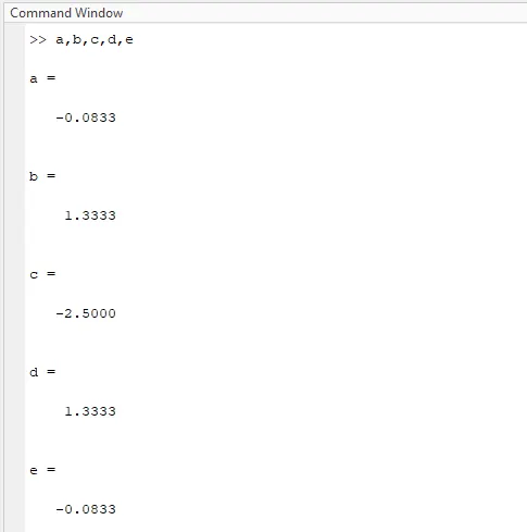
similarly for Skewed right-sided difference and Skewed left-sided difference

Skewed right-sided difference

Taylor table

Stencil	f(i)	`Deltaxf^I(x)`	`Deltax^2f^(II)(x)`	`Deltax^3f^(III)(x)`	`Deltax^4f^(IV)(x)`	`Deltax^5f^(V)(x)`
a f(i)	a	0	0	0	0	0
b f(i+1)	b	b	b/2	b/6	b/24	b/120
c f(i+2)	c	2c	4c/2	8c/6	16c/24	32c/120
d f(i+3)	d	3d	9d/2	27d/6	81d/24	234d/120
e f(i+4)	e	4e	16e/2	64e/6	256e/24	1024e/120
g f(i+5)	g	5g	25g/2	125g/6	625g/24	3125g/120

code

clear all
close all
clc
%right side diff coeff
A=[1 1 1 1 1 1;
    0 1 2 3 4 5;
    0 1/2 4/2 9/2 16/2 25/2;
    0 1/6 8/6 27/6 64/6 125/6;
    0 1/24 16/24 81/24 256/24 625/24;
    0 1/120 32/120 234/120 1024/120 3125/120;];
C=[0;0;1;0;0;0];
B=inv (A)*C;
a=B(1);
b=B(2);
c=B(3);
d=B(4);
e=B(5);
g=B(6);

result

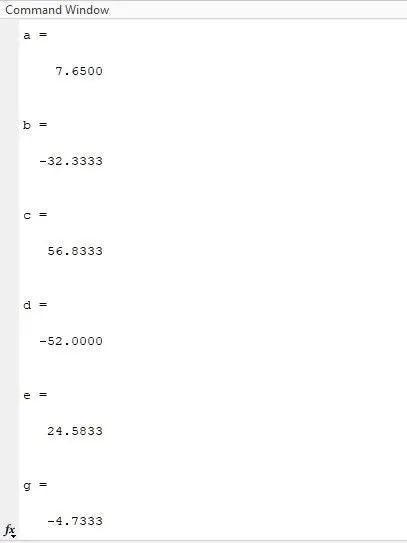
Skewed left-sided difference

Taylor table

Stencil	f(i)	`Deltaxf^I(x)`	`Deltax^2f^(II)(x)`	`Deltax^3f^(III)(x)`	`Deltax^4f^(IV)(x)`	`Deltax^5f^(V)(x)`
a f(i-5)	a	-5a	25a/2	-125a/6	625a/24	-3125a/120
b f(i-4)	b	-4b	16b/2	-64b/6	256b/24	-1024b/120
c f(i-3)	c	-3c	9c/2	-27c/6	81c/24	-234c/120
d f(i-2)	d	-2d	4d/2	-8d/6	81d/24	32d/120
e f(i-1)	e	-1e	e/2	-e/6	e/24	-e/120
g f(i)	g	0	0	0	0	0

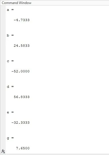
results

clear all
close all
clc

%left side diff coeff
A=[1 1 1 1 1 1;
    -5 -4 -3 -2 -1 0;
    25/2 16/2 9/2 4/2 1/2 0;
    -125/6 -64/6 -27/6 -8/6 -1/6 0
    625/24 256/24 81/24 16/24 1/24 0
    -3125/120 -1024/120 -234/120 -32/120 -1/120 0];
C=[0;0;1;0;0;0];
B=inv (A)*C;
a=B(1);
b=B(2);
c=B(3);
d=B(4);
e=B(5);
g=B(6);

result

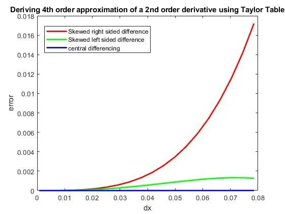
a plot that compares the absolute error between the above-mentioned schemes

to create a plot error we need to calculate absolute err for the three schemes concerning the actual derivative

function program

function [right_sided_differencing] = Skewed_right_sided_difference (x,dx)
A=[1 1 1 1 1 1;
    0 1 2 3 4 5;
    0 1/2 4/2 9/2 16/2 25/2;
    0 1/6 8/6 27/6 64/6 125/6;
    0 1/24 16/24 81/24 256/24 625/24;
    0 1/120 32/120 234/120 1024/120 3125/120;];
C=[0;0;1;0;0;0];
B=inv (A)*C;
a=B(1);
b=B(2);
c=B(3);
d=B(4);
e=B(5);
g=B(6);
right_sided_differencing =(a*(exp(x)*cos(x))+b*(exp(x+dx)*cos(x+dx))+c*(exp(x+2*dx)*cos(x+2*dx))+d*(exp(x+3*dx)*cos(x+3*dx))+e*(exp(x+4*dx)*cos(x+4*dx))+g*(exp(x+5*dx)*cos(x+5*dx)))/(dx^2);
end

function [left_sided_differencing] = Skewed_left_sided_difference (x,dx)
A=[1 1 1 1 1 1;
    -5 -4 -3 -2 -1 0;
    25/2 16/2 9/2 4/2 1/2 0;
    -125/6 -64/6 -27/6 -8/6 -1/6 0
    625/24 256/24 81/24 16/24 1/24 0
    -3125/120 -1024/120 -234/120 -32/120 -1/120 0];
C=[0;0;1;0;0;0];
B=inv (A)*C;
a=B(1);
b=B(2);
c=B(3);
d=B(4);
e=B(5);
g=B(6);
left_sided_differencing =(a*(exp(x-5*dx)*cos(x-5*dx))+b*(exp(x-4*dx)*cos(x-4*dx))+c*(exp(x-3*dx)*cos(x-3*dx))+d*(exp(x-2*dx)*cos(x-2*dx))+e*(exp(x-dx)*cos(x-dx))+g*(exp(x)*cos(x)))/(dx^2);
end

function [central_differencing] = central_differencing_fourth_order(x,dx)
A=[1 1 1 1 1;
    -2 -1 0 1 2;
    2 1/2 0 1/2 2;
    -8/6 -1/6 0 1/6 8/6;
    16/24 1/24 0 1/24 16/24];
C=[0;0;1;0;0];
B=inv (A)*C;
a=B(1);
b=B(2);
c=B(3);
d=B(4);
e=B(5);
central_differencing =(a*(exp(x-2*dx)*cos(x-2*dx))+b*(exp(x-dx)*cos(x-dx))+c*(exp(x)*cos(x))+d*(exp(x+dx)*cos(x+dx))+e*(exp(x+2*dx)*cos(x+2*dx)))/(dx^2);
end

Main program

clear all
close all
clc

%f(x) = sin(x)/x^3
%x = pi/3 for dx range = [pi/4000,pi/40,20]
x=pi/3;
dx=linspace(pi/40,pi/4000,20);
analytical_derivative=-2*sin(x)*exp(x);

for i=1:length (dx)
right_sided_differencing(i)=Skewed_right_sided_difference (x,dx(i));
left_sided_differencing(i)=Skewed_left_sided_difference (x,dx(i));
central_differencing(i)=central_differencing_fourth_order (x,dx(i));
end

for j=1:length (dx)
error_1(j)=abs(right_sided_differencing(j)-analytical_derivative);
error_2(j)=abs(left_sided_differencing(j)-analytical_derivative);
error_3(j)=abs(central_differencing(j)-analytical_derivative);
end
%plot
figure(1)
plot (dx,error_1,'linewidth',2,'Color','r')
hold on
plot (dx,error_2,'linewidth',2,'Color','g')
plot(dx,error_3,'linewidth',2,'Color','b')
xlabel('dx')
ylabel('error')
title('Deriving 4th order approximation of a 2nd order derivative using Taylor Table')
legend('Skewed right sided difference','Skewed left sided difference','central differencing')
hold off

The plot:-Comparing absolute error of central difference scheme skewed right side difference scheme and skewed left side difference scheme.

conclusion

from the obtained result we conclude that

1. Skewed right gives maximum error compared to the other two scheme

2. skewed left side gives error in between the other two scheme

3. Central difference gives the lowest error or it's stable compared to the other two

the central difference gives less error as compared to the skewed right and left side difference, but If we want to calculate error at the boundary, we cannot apply central difference scheme since it requires value from both ends so, in this case, we can apply skewed difference scheme