Week 5 - Rayleigh Taylor Instability

Aim

To study Rayleigh-Taylor Instability and conduct grid independence test.

Introduction

The Rayleigh Taylor instability is an instability of an interface between two fluids of different densities which occur when lighter fluids is pushing heavier fluids.

Eg: Water suspended over fluid in earth gravity, mushroom clouds during volcanic eruptions.

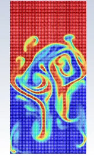
Initially the denser fluid is on top of the lighter fluid at time t=0 and the fluid in static equilibrium and pressure gradient is balanced. As time progress the perturbation starts to develop at the interface and the denser fluids moves downwards due to density while light density fluid pushes the heavy fluid as a result pressure gradient is created. The instabilities result in plumes flowing upwards and spikes flowing downwards. The initial linear phase with small wavelength and amplitudes completely transforms into non-linearity with large irregular wavelength and amplitude. Here the effect of surface tension is neglected.

Theory

• CFD models based on mathematical analysis of Rayleigh Taylor model:

1. Mass diffusion model:

The mass diffusion equation describes the transport of mass and energy due to model viscosity and hence drives actual mixing in the fluids. Even if any configuration is unstable the diffusion process could be responsible for significant mixing if the viscosity is sufficiently large.

2. Single fluid model

Potential flow model

This model is valid for all instability changes from the linear stages through the early non-linear but is limited to Atwood number of 1. In this model the single mode perturbation expands, the flow equation second order around the bubble tips, hence obtaining an ordinary differential equation for the bubble velocity.

2.2 Buoyancy drag model

It is valid for every Atwood number but limited to non-linear stages of the instability.It uses ordinary differential equations to evolve the width of the mixing layer. The bubbles, spikes or amplitude are described by balancing the inertia, buoyancy and drag forces. This model cannot deal with multiple mixing interfaces, cannot be easily extended to two or three dimensions, and as a rule do not address demixing, also known as counter gradient transport ie, reduction of total fluid mass within the mixing zone. To address the above problems two fluids(multi-fluid) models has to be used.

2.3 Besnard-Harlow-Rauenzahn(BHR):

It is more advance version of the single fluid model. The BHR model is based upon the evolution equations arising from second order co relations and gradient-diffusion approximations. Using a mass weighted averaged decomposition, the original BHR model includes the full transport equation for the Reynolds stresses, turbulent mass flux velocity, density fluctuations and turbulent kinetic energy dissipation rate.

3. Multi fluid models

These models use a separate set of equations for each fluid in addition to the main flow equations and provide an accurate modelling framework for demixing by correctly capturing the relative motion of different fluid fragments.

3.1 Two equation K-L turbulence model

The K-L turbulence model involves the equations for turbulent kinetic energy(K) and turbulent length scale(L). The starting point for deriving the model equations are the buoyancy drag models for the self similar growth for RT instabilities.

3.2 Three equation K-L-a turbulence model:

The three equation model was developed as an extension to the two equation K-L model by including a third equation for the turbulent mass flux velocity.

3.3 Four equation K-L-a-b turbulence model

The four equation model was developed as an extension for three equation K-L-a turbulence model by including a fourth equation for the density specific volume covariance. The model can accurately reflect the effect of changes in density fluctuations.

• What is Atwood number? What is its effect on Rayleigh Taylor instability?

Atwood number(A) is a dimensionless number in fluid dynamics used in the study of hydrodynamic instabilities in density stratified flows. It is defined as:

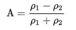
ρ1- density of heavy fluid

ρ2- density of light fluid

Case1: A= (998.2-1.225)/(998.2+1.225) = 0.9975

Case2: A= (998.2-400) / (998.2+400) = 0.4278

• Can we solve the problem using steady state approach.

The solution to a problem using steady state solver is used when the desired result is when the system achieved steady state. When the system variables under consideration is time dependent then it is better to use transient state solver for capturing the time dependence of the problem. In case of problem like Rayleigh Taylor instability the instability grows exponentially at each time step.Hence it is better to use a transient solver.

Solving and modelling Approach

• For studying Rayleigh Taylor Instability a 2D model is considered.
• In Spaceclaim a square 20mm*20mm is created and is coverted to surface using pull tool.
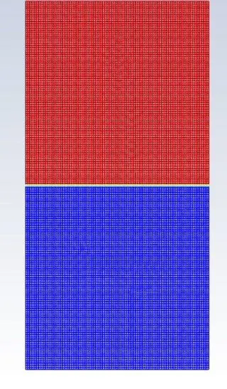
• Another square of same dimension is created above the first and converted to surface. The below square represent air and the top one water.
• From workbench menu share topology is enabled so that a conformal mesh will be created.
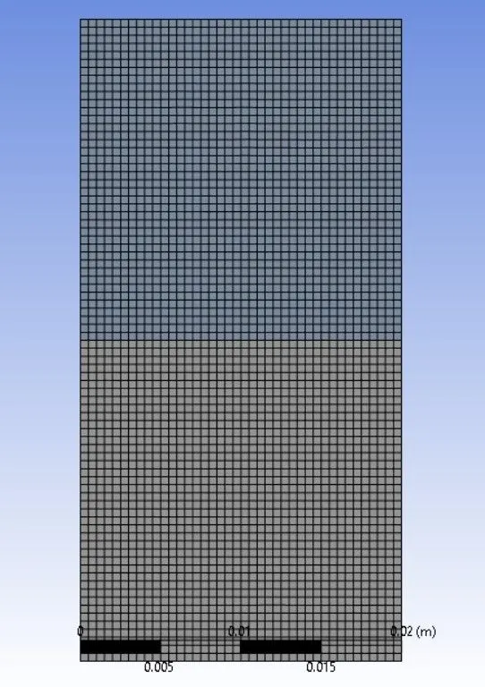
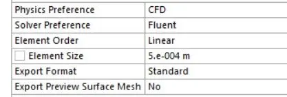
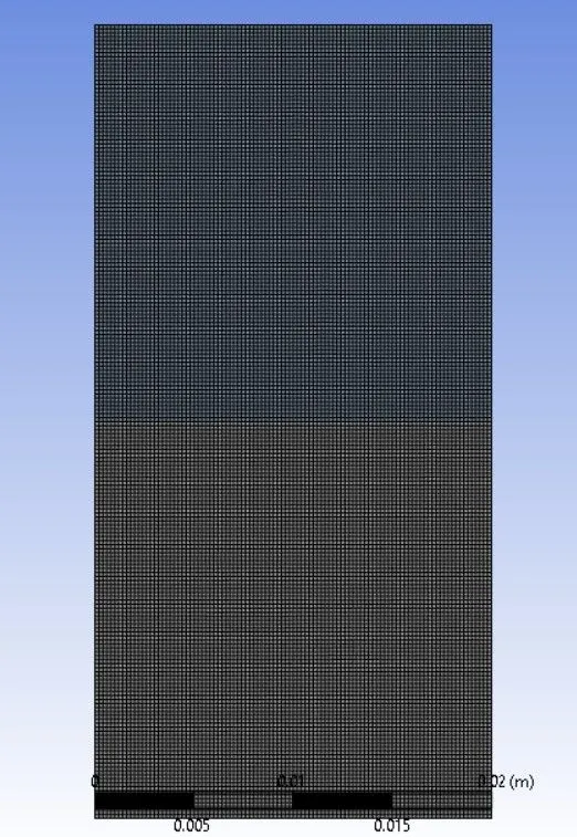
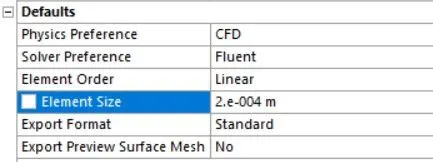
• Create a mesh with an element size of 0.5mm, this will be the base line mesh.
• In setup use a pressure based solver with absolute velocity formulations and transient solver in order to visualize how the interface collapses as a function of time.
• Gravity is enabled and a value of -9.81m/s2 is typed in the space against y since the geometry is aligned in the xy plane.
• Laminar viscous model is used and multi phase model is selected with 2 Eulerian phases in implicit mode.
• Add water to the materials and go to list phases: set primary phase as air and secondary phase as water.
• The setup is standard initialized and click on patch.
• Inside patch select water from phase and put in volume fraction, select water surface and put in value of water to one.
• Similarly for air surface put in an air value of zero.
• Create a new contour and plot for volume fraction , also setup animation.
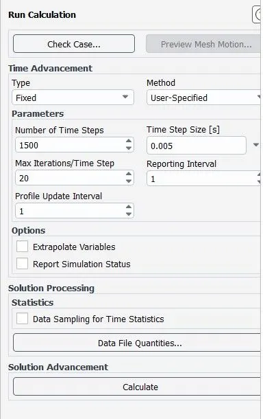
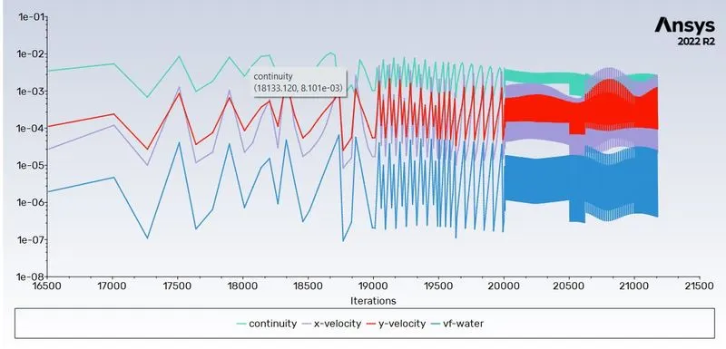
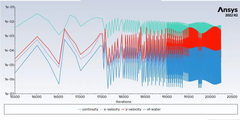
• From run calculation set time stepping method as fixed with a time step size of 0.005 and number of iterations to 1500.
• Hit calculate.

Pre-processing and solver settings

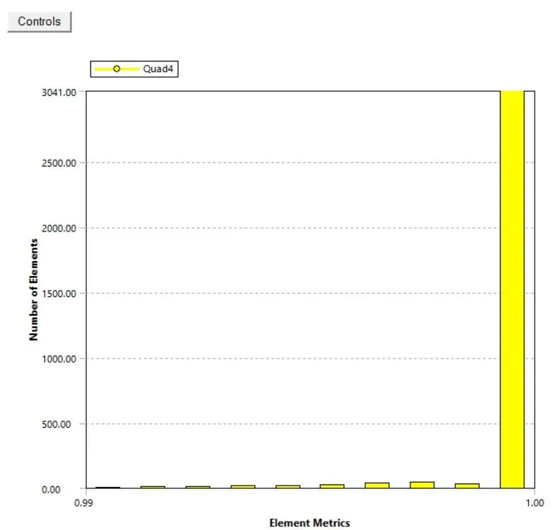
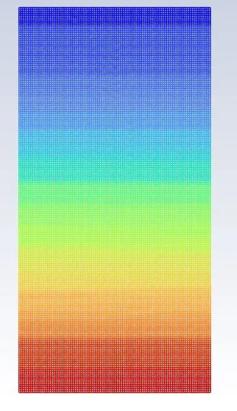
Mesh details and setup for baseline mesh

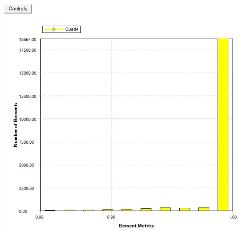
Refined mesh

Air properties:

Density : 1.225 kg/m3

Viscosity: 1.789e-5 Pa-s

Water properties:

Density : 998.2 kg/m3

Viscosity:0.001003 Pa-s

User material properties:

Density : 400 kg/m3

Viscosity: 0.001 Pa-s

Results:

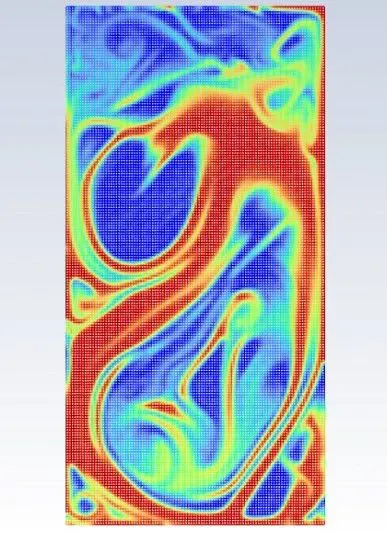
Baseline mesh:

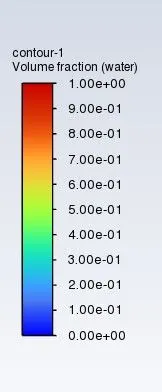
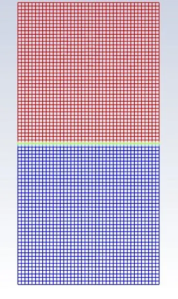
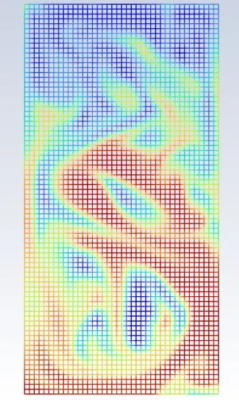
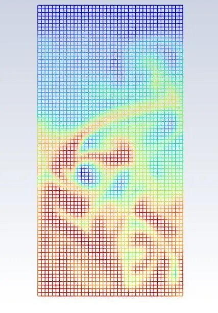
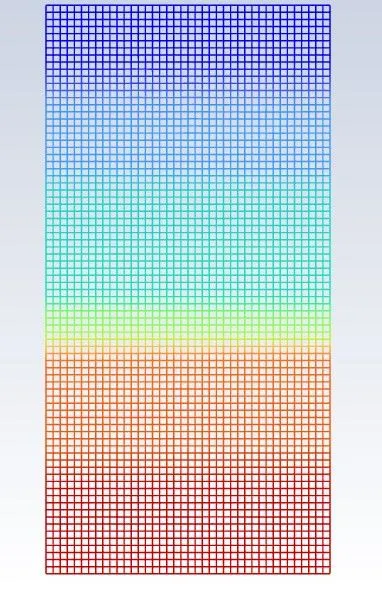
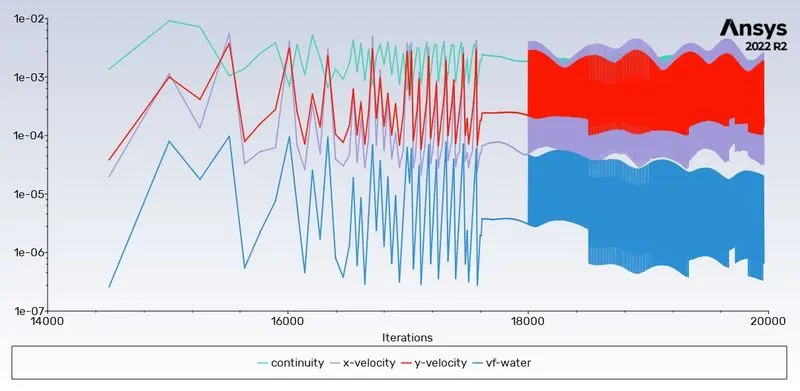
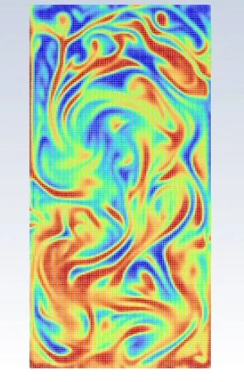
Refined mesh

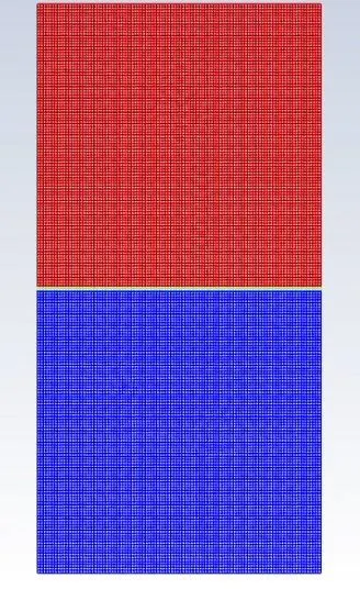
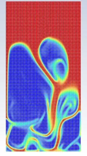
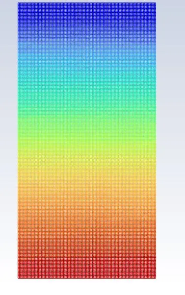
User materials

Conclusion

• Visualised the Rayleigh Taylor Instability using baseline mesh, a refined mesh with air and water as material and using water and a user defined material the properties of which is mentioned above using refined mesh.
• The interface thickness of the refined mesh is smaller than that of the baseline mesh hence it gives better result.
• The variation of Atwood number has a direct impact on the progression of the instability, it’s amplitude and wavelength.
• Finer mesh and small time steps gives good result.

Link to animation:https://drive.google.com/drive/folders/1O7TidYBSFEwRNGmlfnysOfNWZhhilWct?usp=sharing