Week 4 - CHT Analysis on Exhaust port

Aim

To perform conjugate heat transfer analysis on an exhaust port with four inlet and single outlet.

Objectives

1. Give a brief description of why and where a CHT analysis is used.
2. Maintain the y+ value according to the turbulence model and justify the results.
3. Calculate the wall/surface heat transfer coefficient on the internal solid surface & show the velocity & temperature contours in appropriate areas.
4. How would you verify if the HTC predictions from the simulations are right? On what factors does the accuracy of the prediction depend on?(Answer in conclusion)

Introduction and theory

1. Why and where a CHT is used?

Conjugate heat transfer is a type of heat transfer analysis between solids and fluid(s). This type of heat transfer includes both convection (between fluids) and conductive (between solids) heat transfer, as well as both forced and natural convection. Common applications and use cases of this thermal simulation type include electronics cooling, heat exchangers, industrial machinery etc.

Due to the fluid motion, three contributions to the heat equation are included:

1. The transport of fluid implies energy transport too, which appears in the heat equation as the convective contribution. Depending on the thermal properties on the fluid and on the flow regime, either the convective or the conductive heat transfer can dominate.
2. The viscous effects of the fluid flow produce fluid heating. This term is often neglected, nevertheless, its contribution is noticeable for fast flow in viscous fluids.
3. As soon as a fluid density is temperature-dependent, a pressure work term contributes to the heat equation. This accounts for the well-known effect that, for example, compressing air produces heat.

2. Y+ and it’s relation with turbulence model

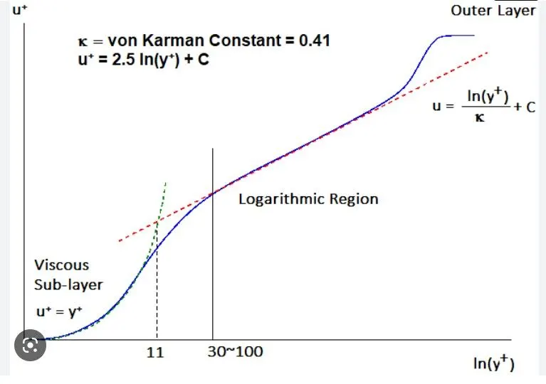
Y+ is used to distinguish different regions near the wall or in viscous region. In order to resolve the viscous sub layer the size of the mesh should be small and mesh should be dense near the wall. Based on the y+ value the size of the first layer can be calculated.

The k-epsilon model is used where flow does not demand to integrate the solution over the sub layer and wall bounded effects are secondary. For such cases the first cell can be kept away at y+ 30-300. In such scenario sub-layer and buffer layer is not resolved instead semi empirical formulas called called wall function are used to bridge the viscosity affected region between the wall and fully turbulent region.

In the exhaust port simulation by using proper mesh refinement techniques like adding inflation layers as well as reducing the element size the desired value of the y plus is maintained.

Solving and modelling Approach

• Load the solid geometry to Spaceclaim, change the units to m.
• Extract the fluid volume using volume extract tool in prepare, remove duplicate edges if any by using repair tool.
• Move the solid volume and fluid volume to a new component and enable SHARE from workbench.
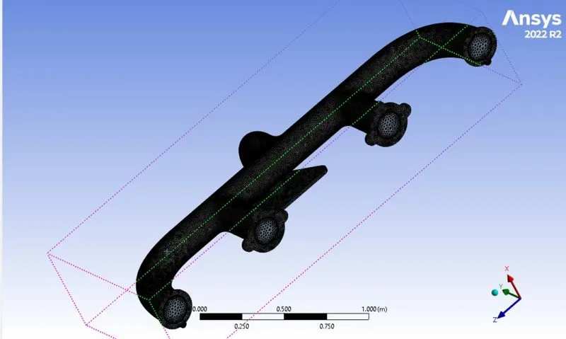
• In the meshing option create a baseline mesh to check for any interference or overlap.
• Name different parts like inlets, outlets and walls using face selection tool.
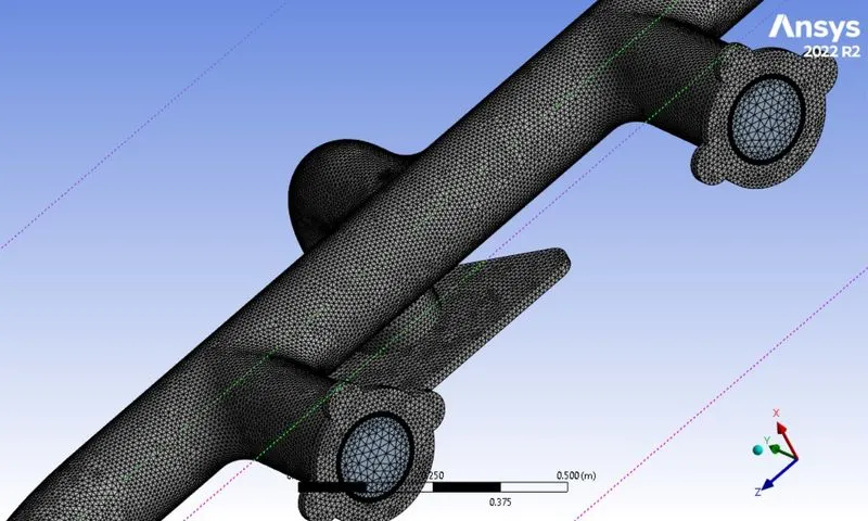
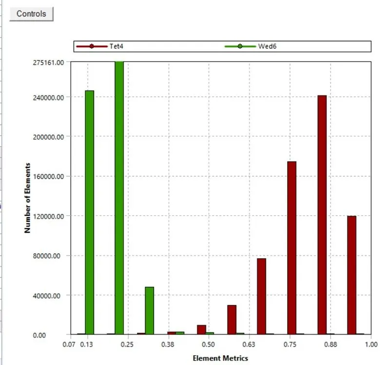
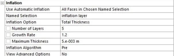
• In order to add inflation layers to the fluid volume select the fluid surface and add inflation layers from mesh options.
• Here maximum thickness option is used for creating inflation layers and 5mm is set as the maximum thickness.
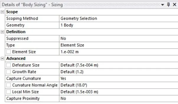
• The solid volume mesh is refined by making use of the body sizing tool and reducing the element size to 10mm and turn on the capture curvature option.
• For solving a pressure based solver with absolute velocity formulation under steady state is used.
• Energy check box is turned on since we are also required to solve energy equation since temperature is involved.
• K-epsilon viscous model with standard wall function is selected.
• Fluid material is kept air and solid material is kept aluminium.
• Inlet velocity is 5m/s and temperature 700 K.
• Assign h=20w/m2K to the outer wall.
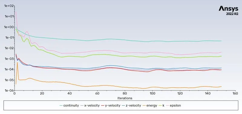
• Hybrid initialization is used and the setup is run for 150 iterations.
• Velocity contour temperature contour and heat transfer coefficient is created.

Preprocessing and solver techniques

Results

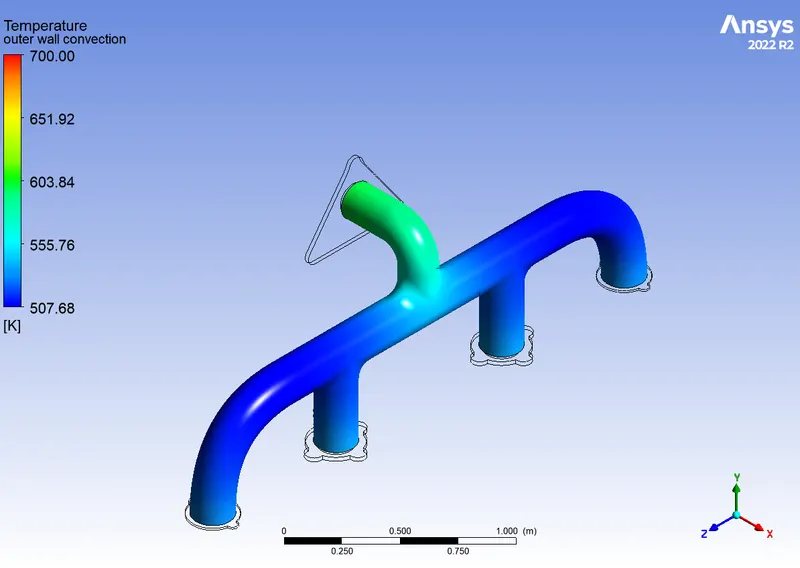
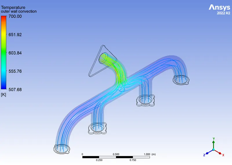
1.Temperature contour with and without streamline

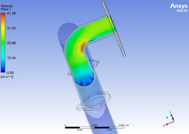
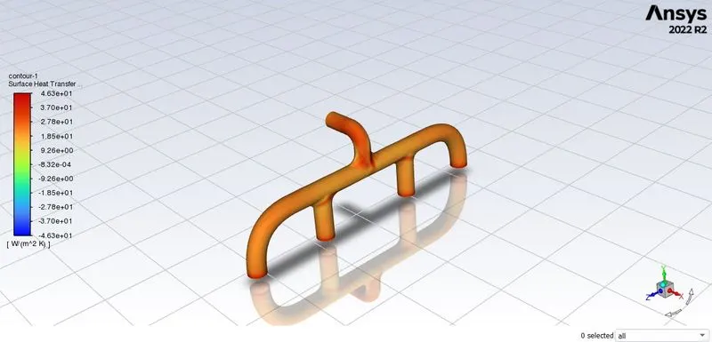
2.Velocity contour at outlet pipe and heat transfer coefficient contour

3.Residuals

Conclusion

• The heat transfer coefficient is proportional to the Reynolds number and the dependence varies for Laminar and turbulent flows.
• Due to conservation of mass the velocity at the outlet pipe is greater than the inlet pipes, hence Reynolds number as well as heat transfer coefficient is maximum at the outlet pipe walls.
• For mapping this heat transfer coefficient inflation layers are added to the fluid volume surface since heat transfer coefficient is calculated at the interface of the solid and the fluid.
• For capturing inflation layer thickness has to be calculated according to the yplus value for the model used.
• The temperature contour shows that the solid wall temperature is higher for the outlet pipe , this is because of the higher value of heat transfer coefficient at the outlet.
• The heat transfer coefficient predicted by the simulation can be verified by calculating the heat transfer values directly using standard results like Dittus-Boelter equation.
• The heat transfer coefficient prediction depend upon the use of proper mesh size near the walls since this is calculated at the interface. So consideration have to be made to the yplus value for this calculation keeping in mind the wall function corresponding to the viscous model used.