Week 5 - Rayleigh Taylor Instability

AIM: Perform the Rayleigh Taylor instability simulation for 2 different mesh sizes with the base mesh being 0.5 mm. Run one more simulation with water and user-defined material(density = 400 kg/m³, viscosity = 0.001 kg/m-s) for refined mesh.

INTRODUCTION:

Rayleigh-Taylor instability is an instability of an interface between two fluids of different densities which occurs when the the ligther fluid is pushing the heavier fluid.the equilibrium here is unstable to any perturation or disturances of the interface.

THEORY:

Rayleigh-Taylor instability is a phenomena in the which heavier fluid is superposed over a ligthter one in a gravitational field where the fluid interface is unstable. Any perturbation of the this interface will in general develop with time, exhibiting the penetration of both heavier and ligther fluids into one another.if a parcel of heavier fluid is displaced with an equal volume of ligther fluid displaced upwareds,This RT instability due to the gravitational field was initially proposed by Rayleigh and subsequently has been applied to all fluids by taylor.

This is same like mushroom clouds like those from volcanic eruption and atmospheric nuclear explosions.

Q1. What are some practical CFD models that have been based on the mathematical analysis of Rayleigh Taylor waves? In your own words, explain how these mathematical models have been adapted for CFD calculations.

Atwood number: is a dimensionless number in fluid used in the study of hydrodynamic instabilities in density stratified flows. It is a diamensionless density ratio defined as. where = density of heavier fluid =density of ighter fluid.

Atwood number =(heavier fluid density - lighter fluid density)/(heavier fluid density + lighter fluid density)

Atwood number lies between 0 to 1.

Multi fluid models:

multi fluid models are separate set of equations for each fluid addition to the main flow equation to provide accurate modelling informaton.

1 Two equation K-L turbulance model: In this turbulance model involves equation for turbulant kinetic energy K and turbulant length scale L.

2 Three equation K-L-a turbulance model: In this equation was developed an extension to the two equation k-L model by adding a third equation for turbulance mass flux velocity.

3 Four equation K-L-a-b turbulance model: In this equation developed an extension of third equation by adding fourth equation for density specific volume covariance.

SLOVING AND MODELLING APPROACH:

1.First i open the workbench and then i drag the anasys fluent into the work space. then i open then geometry on the popup and i open the spaceclaim and import the geometry into the spaceclaim.

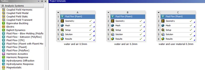
fig:setup window

2.then i made square with 20*20m for water and i convert into 3D by pull command option, then i created another one for air with same dimensions and i converted into 3D. then i used command share tropology.

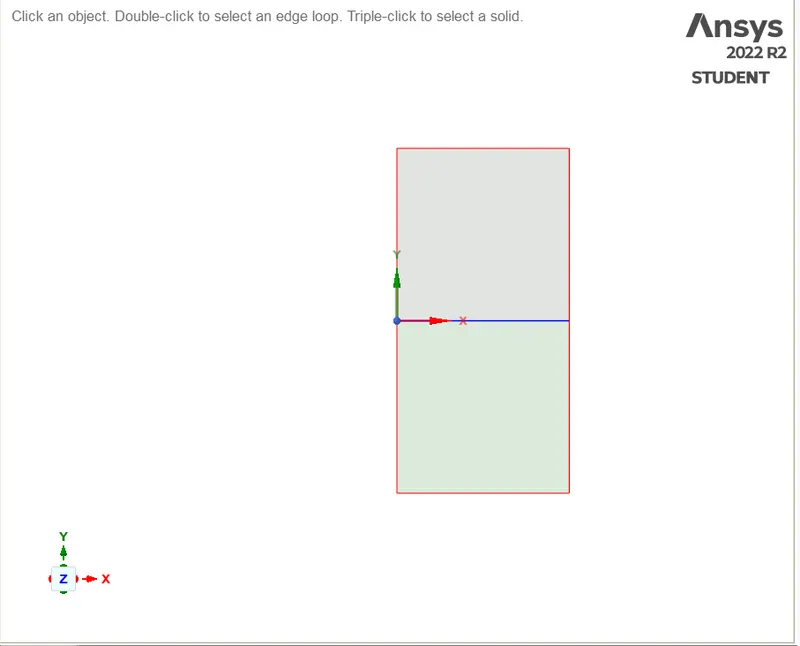
fig:geometry

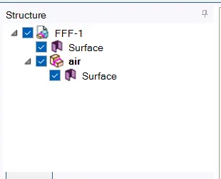
fig:gemetry setup.

3.then i went to the meshing part to make mesh on the geometry with the 0.5mm and 0.3mm.

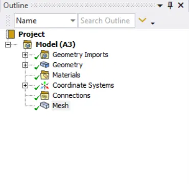
fig:mesh setup.

case 1 mesh size with 0.5mm water and air.

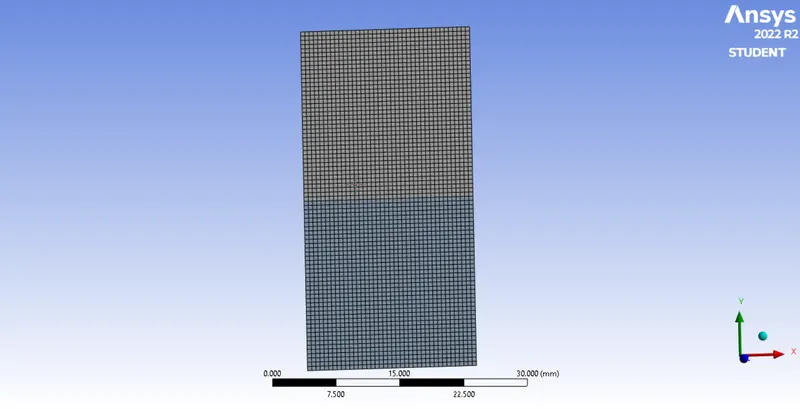
fig:meshed geometry of 0.5mm.

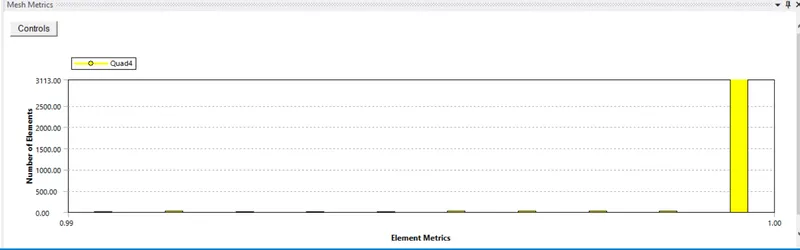
fig: mesh quality.

case 2 mesh size with 0.3mm water and air.

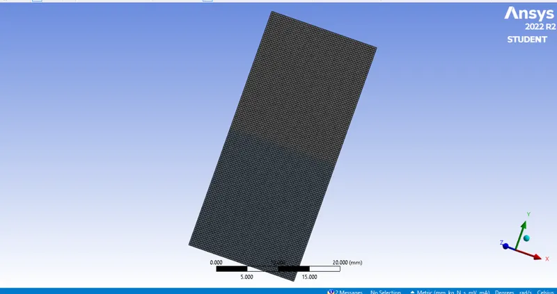
fig:meshsize 0.3mm.

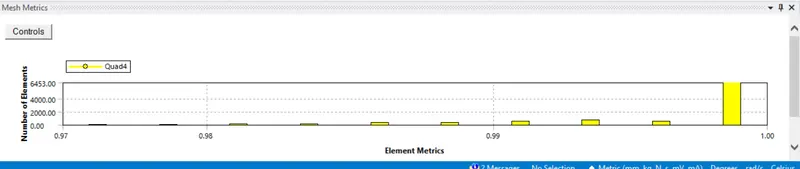
fig: mesh quality.

case 3 mesh size with 0.3mm water and user material i.e density = 400 kg/m³, viscosity = 0.001 kg/m-s.

fig:mesh size 0.3mm

fig:mesh quuality.

4.then i went to the solver setup to give the input conditions to run the simulation. here i have given the boundary condition like input fluids has air and water for case 1 and 2. for case 3 water and user define material that is properties density = 400 kg/m³, viscosity = 0.001 kg/m-s.

5.then i went to the multphase and here i have set the volume of fraction and i set the domains for air and water. then i initialized the simulation and i went for the patching here i set water for 1 and air for 0, for the case water for one and user define material of zero.

6.then i have created the report for the volume fraction, contour plot for the volume fraction and also i have made animations for each time steps.

OUTPUT:

CASE 1

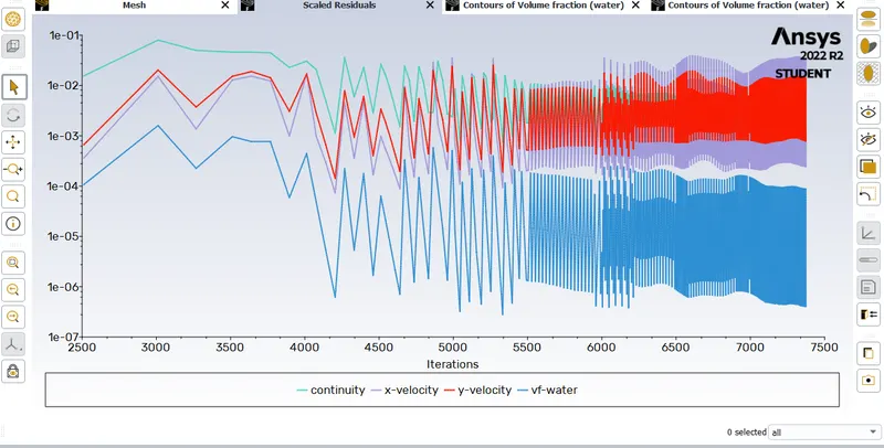
fig: Residual plot.

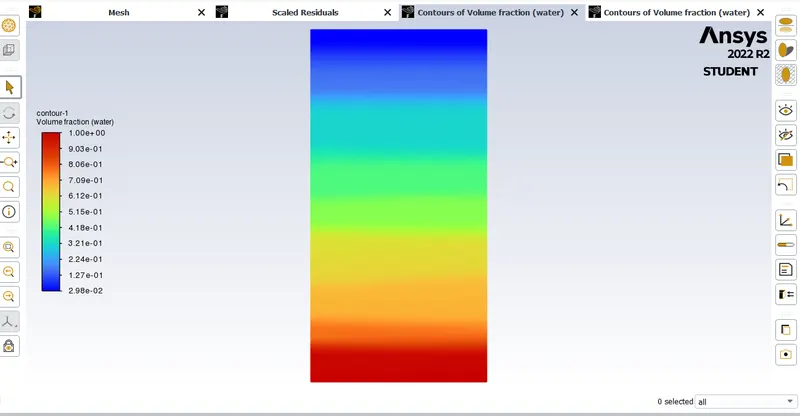
fig:volume fraction of the stable stage.

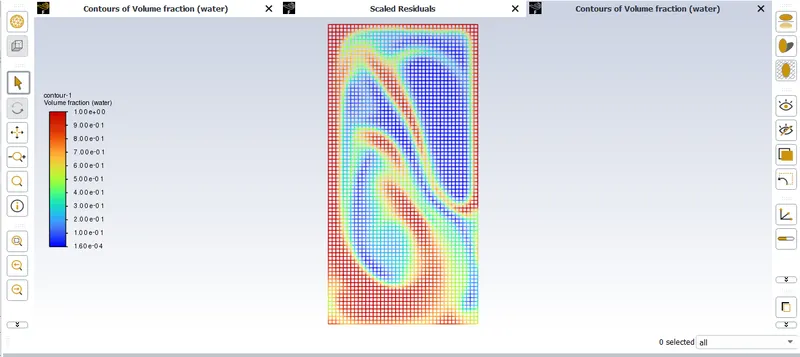
fig:volume of fraction at middle.

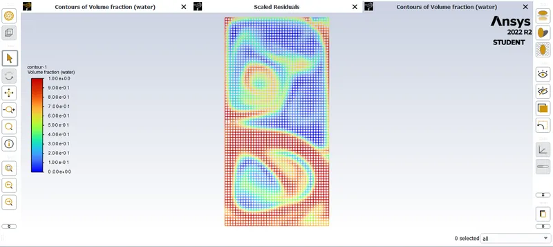
fig:volume of fraction of middle.

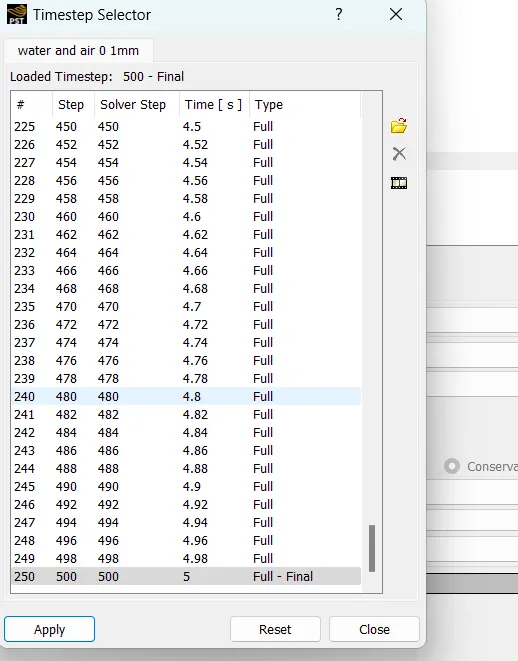
fig:time steps.

CASE 2

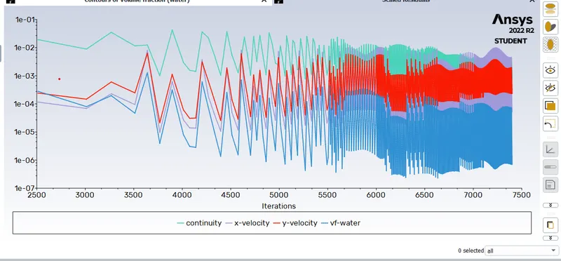
fig:Residual plot

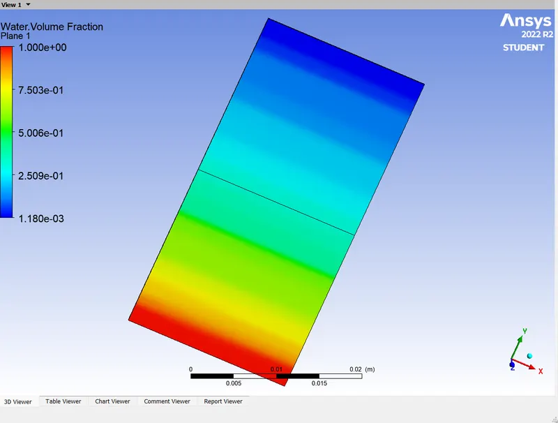
fig:volume of fraction final stage.

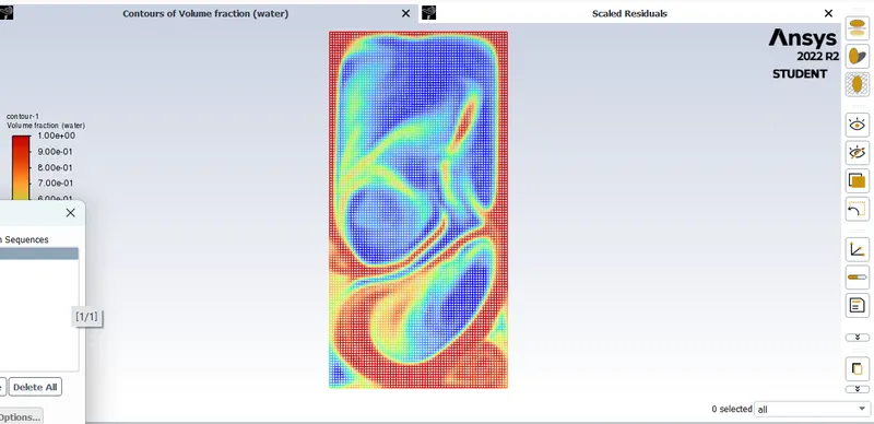
fig:volume of fraction of middle stage.

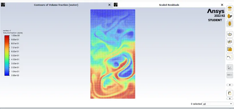
fig: volume of fraction at middle stage.

fig: Time steps.

CASE 3

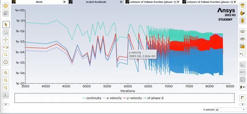
fig: residual plot.

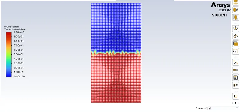
fig: volume of fraction at stage one.

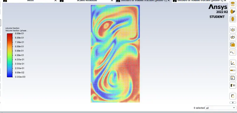
fig: volume of fraction at middle.

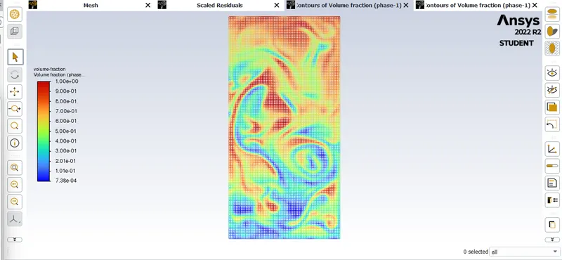
fig: volume of fraction at meddle.

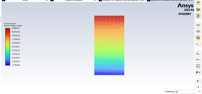
fig: volume of fraction at stable.

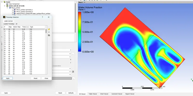
fig:time steps.

Q2. Explain why a steady-state approach might not be suitable for these types of simulation?

Here in this study, the instabilities information is sensitive and completely time-dependent. At each and every time step, the instabilities grow exponentially. Thugh steady state simulation is capable t capture those instabilities but the result would not be time accurate. Anyways transient state calculation with reduced time-steps can capture these instabilities at each an every time-steps and it gives accurate time dependent results.

CALCULATIONS:

Atwood number=(ρ1-ρ2)/ρ1+ρ2)

ρ1= water density

ρ2=user define material density

ρ1=1000 kg/m³

ρ2=400 kg/m³

Atwood number=1000-400/1000+400=0.428571.

RESULT:

https://drive.google.com/file/d/1XVd_eyBhnCToMyowyarYiSR693iNJt4R/view?usp=share_link

CONCLUSION:

here i conclued that the penetration speed is dependent on the density differenace between ligther fluid and heavier fluid.

the mesh size capture the accurate result in the peneration of the fluid motion. if the density different is small the motion of the penetration of the fluid motion is slow and if density different is high then the penetration motion is high.