Week 5 - Rayleigh Taylor Instability

Rayleigh Taylor Instability

AIM:-

To discuss Rayleigh Taylor instability and to Perform the simulation of it for 2 different mesh sizes.

OBJECTIVES:-

• To explain some practical CFD models that are based on the mathematical analysis of Rayleigh Taylor waves and how these mathematical models are adapted for CFD calculations.
• To perform the Rayleigh Taylor instability simulation for 2 different mesh sizes with the base mesh being 0.5 mm.
• To compare the results by showing the animations and to explain the effect of mesh size on simulation.
• To run one more simulation with water and user-defined material(density = 400 kg/m³, viscosity = 0.001 kg/m-s) for refined mesh.
• To define the Atwood Number and to find out the Atwood number for both the cases and explain how the variation in Atwood number in the above two cases affects the behavior of the instability.

INTRODUCTION:-

Rayleigh-Taylor instability (RTI) is the interpenetration of two fluids of different densities that occurs whenever a light fluid pushes on a heavy fluid. It is a dynamic process whereby the two fluids seek to reduce their combined potential energy.. It can occur under gravity and, equivalently, under an acceleration of the fluid system in the direction toward the denser fluid. A simple example may illustrate typical evolution times for the overturn of ordinary liquids under the effect of the earth's gravity. Assuming an acceleration a = 9.8 m/s 2 and a perturbation wavelength A = 1 cm, the classical e-folding time r = X/A/V~rra of the free-surface RT instability would be 0.013 s. Even if an unstable equilibrium would be established, the instability evolution would be too fast for direct observation. However, the typical finger-like flow patterns can be nicely modeled, for instance, by Hele-Shaw cells consisting of thin sheets of viscous fluids inside the gap between two parallel glass plates.

Examples include the behavior of water suspended above oil in the gravity of Earth , mushroom clouds like those from volcanic eruptions and atmospheric nuclear explosions, supernova explosions in which expanding core gas is accelerated into denser shell gas, instabilities in plasma fusion reactors and inertial confinement fusion.

This situation has engineering implications in several industries. For example in die casting, liquid metal is injected in a cavity filled with air. In poor designs or other situations, some air is not evacuated and stay in small cavity on the edges of the shape to be casted. Thus, it can create a situation where the liquid metal is above the air but cannot penetrate into the cavity because of instability. This instability deals with a dense, heavy fluid that is being placed above a lighter fluid in a gravity field perpendicular to interface. Example for such systems are dense water over oil (liquid–liquid), or water over air(gas–liquid).

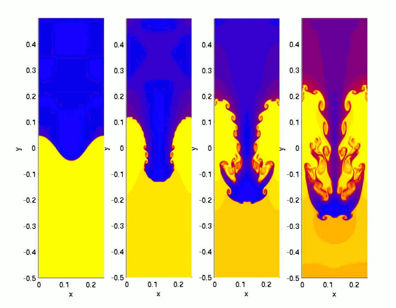
Hydrodynamics simulation of a single "finger" of the Rayleigh–Taylor instability is shown below

Practical CFD models that are based on the mathematical analysis of Rayleigh Taylor waves

Kelvin–Helmholtz instability

It typically occurs when there is velocity shear in a single continous fluid, or additionally where there is a velocity difference across the interface between two fluids. The theory predicts the onset of instability and transition to turbulent flow within fluids of different densities moving at various speeds.The Kelvin-Helmholtz instability phenomena is an all encompassing occurrence of fluid flow seen time and time again in nature. From the waves of the ocean to the clouds above in the sky, the Kelvin-Helmholtz instability is responsible for some of nature's most basic structures. Further analysis and modeling of the Kelvin-Helmholtz instability can result in an understanding of the worlds natural phenomena and more.

Plateau–Rayleigh instability

It explains why and how a falling stream of fluid breaks up into smaller packets with the same volume but less surface area. It is part of a greater branch of fluid dynamics concerned with fluid thread breakup. The explanation of this instability begins with the existence of tiny perturbations in the stream.These are always present, no matter how smooth the stream is (for example, in the liquid jet nozzle, there is vibration on the liquid stream due to a friction between the nozzle and the liquid stream).

Richtmyer–Meshkov instability (RMI)

It occurs when two fluids of different density are impulsively accelerated. Normally this is by the passage of a shock wave. The development of the instability begins with small amplitude perturbations which initially grow linearly with time. This is followed by a nonlinear regime with bubbles appearing in the case of a light fluid penetrating a heavy fluid, and with spikes appearing in the case of a heavy fluid penetrating a light fluid. A chaotic regime eventually is reached and the two fluids mix.

PROCEDURE:-

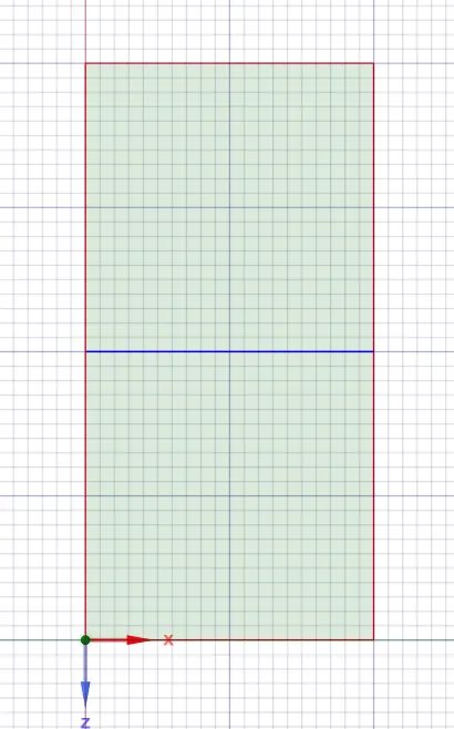
Geometry:- 2 components are created using surface pull option each of 20mm X 20mm sharing a common edge.

CASE 1:- Baseline mesh

Meshing:-

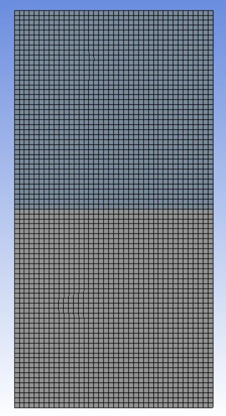
• Here basic quad mesh is generated.

Element size	0.5mm
Number of nodes	3321
Number of elements	3200

Setup:-

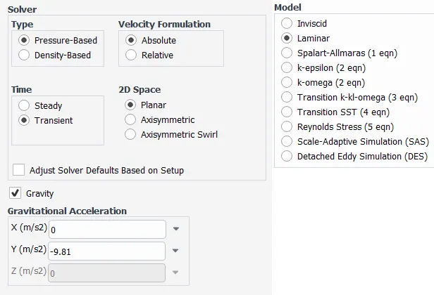
• Here we need to setup a solver the solver type is pressure based tansient state and absolut velocity formation.
• After the solver setup we need to select the laminar flow model.

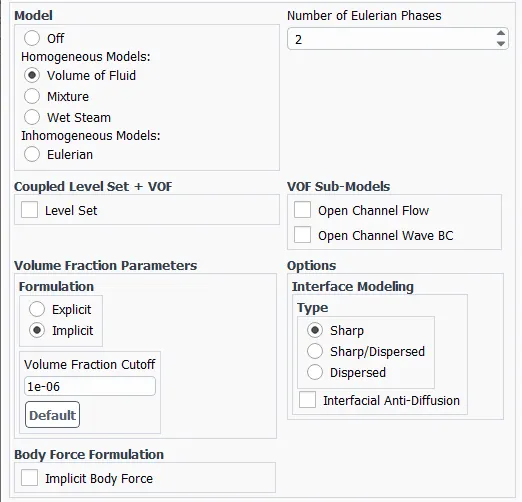
• Here we have taken two different fluids water and air so this simulation comes under Multiphase modeling method. Then we need to select volume of fluid homogeneous model and implicit formulation.

Boundary conditions:-

After selecting the viscous and multiphase model we need to set a boundary conditions.

Fluids

• Air:-

Density=1.225 kg/m^3

Kinematic viscosity= 1.789e-5 kg/ms

• Water:-

Density= 998.2 kg/m^3

Kinematic viscosity= 0.001003 kg/ms

Gravity= -9.81 m/s^2 (Y-axis)

RESULTS:-

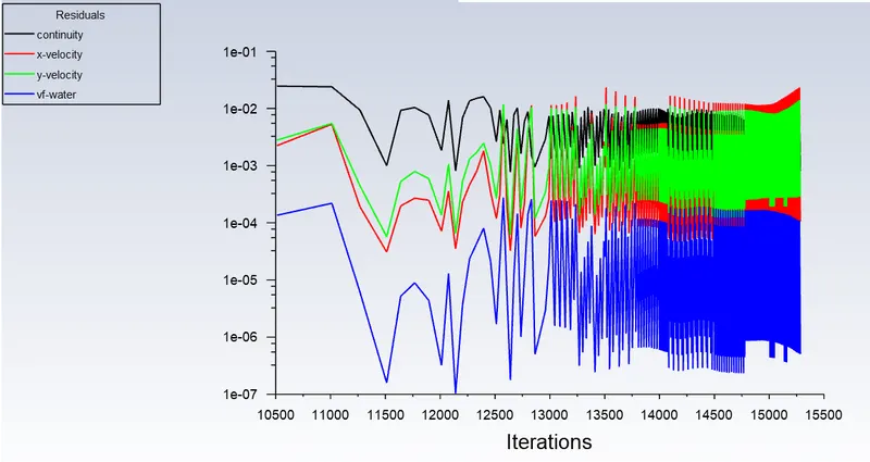
Residuals plot:-

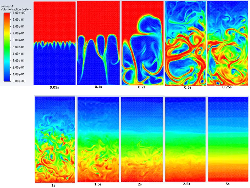
Contours:-

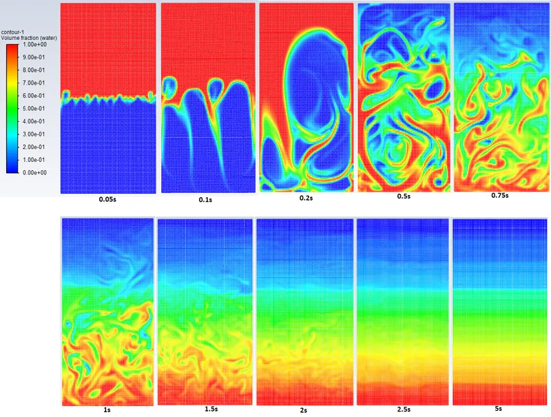
CASE 2:- Mesh size= 0.25mm

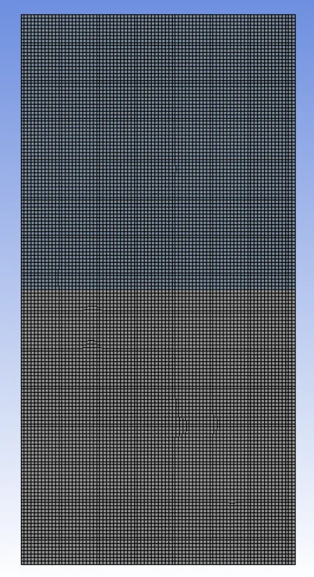
Meshing:-

Element size	0.25mm
Number of nodes	13041
Number of elements	12800

Setup :-

• Here we need to setup a solver the solver type is pressure based tansient state and absolut velocity formation.
• After the solver setup we need to select the laminar flow model.
• Here we have taken two different fluids water and air so this simulation comes under Multiphase modeling method. Then we need to select volume of fluid homogeneous model and implicit formulation.

Boundary conditions:-

After selecting the viscous and multiphase model we need to set a boundary conditions.

Fluids

• Air:-

Density=1.225 kg/m^3

Kinematic viscosity= 1.789e-5 kg/ms

• Water:-

Density= 998.2 kg/m^3

Kinematic viscosity= 0.001003 kg/ms

Gravity= -9.81 m/s^2 (Y-axis)

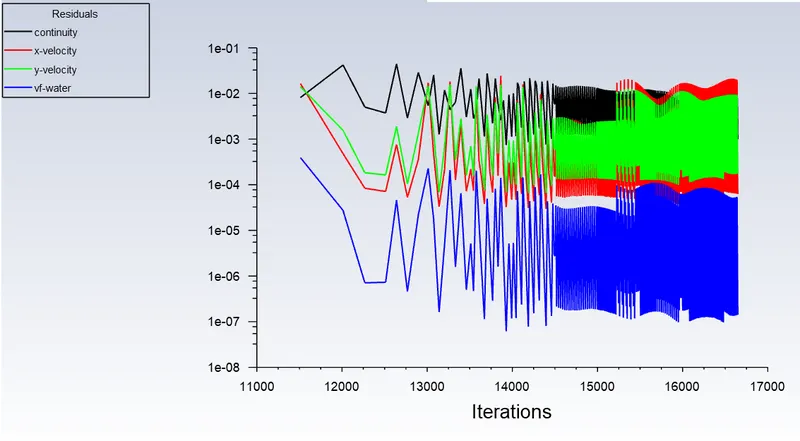
Results:-

Residuals plot:-

contours:-

CASE 3:- Mesh size= 0.1mm

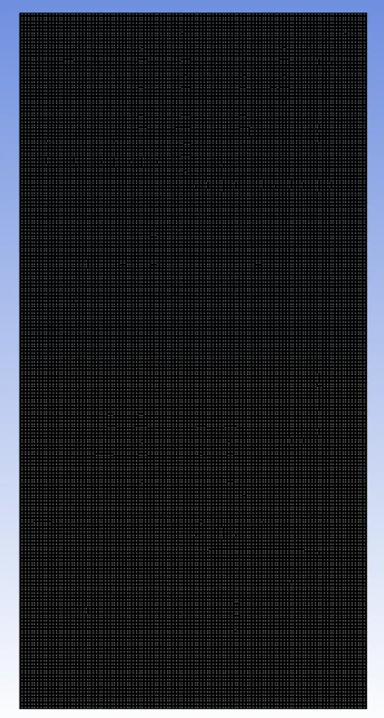
Meshing:-

Element size	0.1mm
Number of nodes	80601
Number of elements	80000

Setup :-

• Here we need to setup a solver the solver type is pressure based tansient state and absolut velocity formation.
• After the solver setup we need to select the laminar flow model.
• Here we have taken two different fluids water and air so this simulation comes under Multiphase modeling method. Then we need to select volume of fluid homogeneous model and implicit formulation.

Boundary conditions:-

After selecting the viscous and multiphase model we need to set a boundary conditions.

Fluids

• Air:-

Density=1.225 kg/m^3

Kinematic viscosity= 1.789e-5 kg/ms

• Water:-

Density= 998.2 kg/m^3

Kinematic viscosity= 0.001003 kg/ms

Gravity= -9.81 m/s^2 (Y-axis)

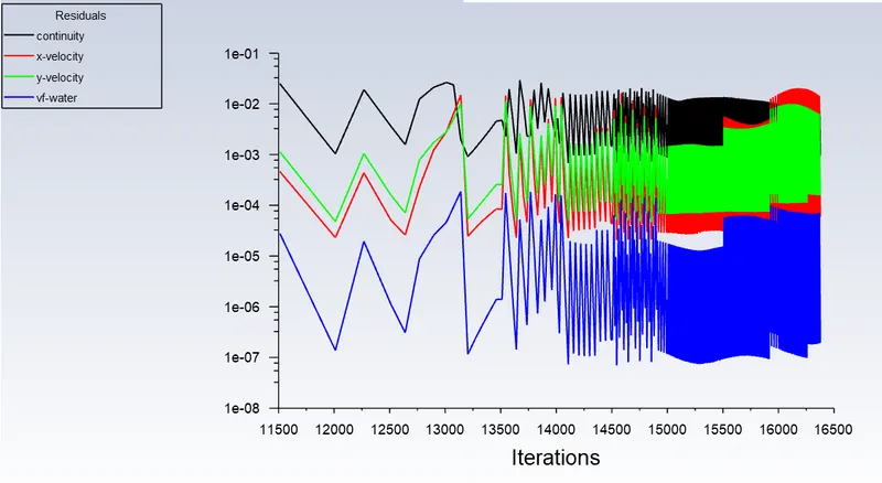
Results:-

Residuals plot:-

Contours:-

CASE 4:- User-defined material for refined mesh.

Setup :-

• Here we need to setup a solver the solver type is pressure based tansient state and absolut velocity formation.
• After the solver setup we need to select the laminar flow model.
• Here we have taken two different fluids water and air so this simulation comes under Multiphase modeling method. Then we need to select volume of fluid homogeneous model and implicit formulation.

Boundary conditions:-

After selecting the viscous and multiphase model we need to set a boundary conditions.

Fluids

• Air:-

• Density=400kg/m^3

  Kinematic viscosity= 0.001kg/ms

• Water:-

• Density= 998.2 kg/m^3

  Kinematic viscosity= 0.001003 kg/ms

  Gravity= -9.81 m/s^2 (Y-axis)

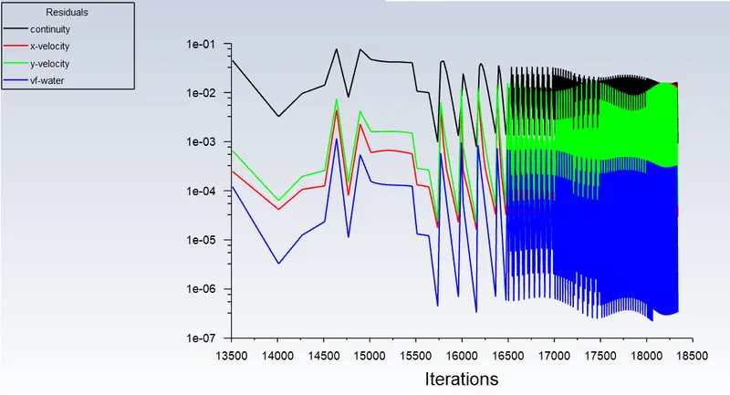
Results:-

Residuals plot:-

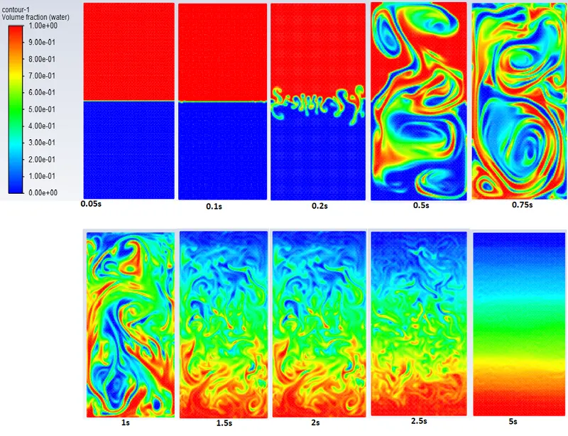
Contours:-

CONCLUSION:-

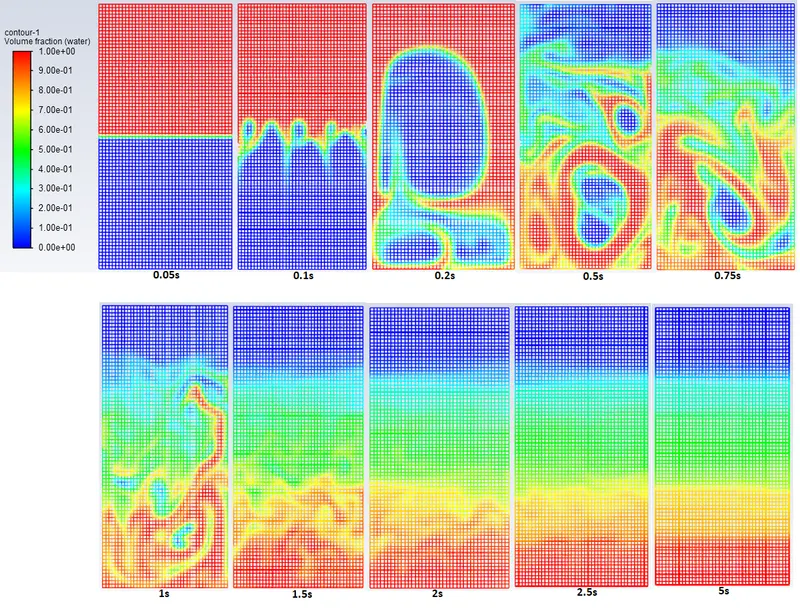
• It is observed that as we refine the mesh that is as we decrease the element size the simulation results gets smoother about the irregularities and instability that takes place at interface of two fluids.
• When we compare the water-air interface and water-user defined interface we can observe that in water - air interface there is a sudden spike formation and bubbles in very initial stage itself when two fluids interacts with each other,
• whereas in water - userdefined interface there is a delay in formation of spikes and bubbles, it is formed in third stage as we can see in the above results. It is because the density and viscocity of the user defined material is greater than the air.
• Rayleigh Taylor Instability can be seen clearly when the the lighter fluid is pushing the heavier fluid.

Why a steady-state approach not suitable for these types of simulation?

• Steady-state simulation computes the fully developed solution that does not change in time and it directly gives the final results of the solution Whereas, Transient simulation computes the instantaneous values in each time for each quantity.
• In RT instability we acctualy need a transient state when two fluids of different density interacts with each other the changes in the solution and formation of spikes, bubbles, vortex can only captured in transient state.

Atwood Number

The Atwood number (A) is a dimensionless number in fluid dynamics in used in the study of hydrodynamic instabilities in density stratified flows. It is a dimensionless density ratio defined as

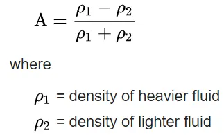
For water - air domain the Atwood number (A) is = 0.9975

For water - user defined domain the Atwood number (A) is = 0.42775

• For Atwood number (A) is closer to 1 means lighter fluids below heavier fluid takes the form of larger bubbles, and clear formation of bubbles.
• when A is not close to 1 then it is difficult to differentiate between spikes and bubbles because of low density.