Mixing efficiency

MIXING EFFICIENCY

AIM:

To set up steady state simulations and to compare the mixing effectiveness of short and long tee when hot inlet temperature is 36°C and the cold inlet is at 19°C for the different cases.

OBJECTIVE:

• To compare the RANS based turbulence model K-epsilon and K-omega.
• To compare cell count,average outlet temperature,number of interations for convergence in a table.
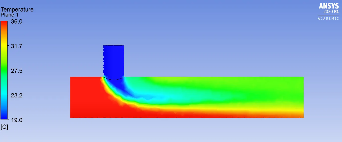
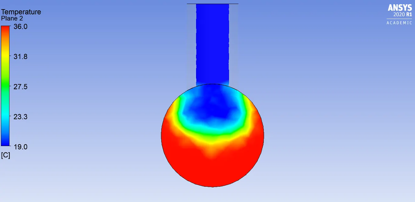
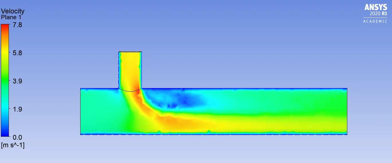
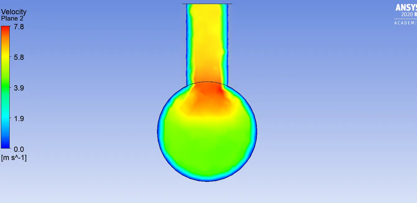
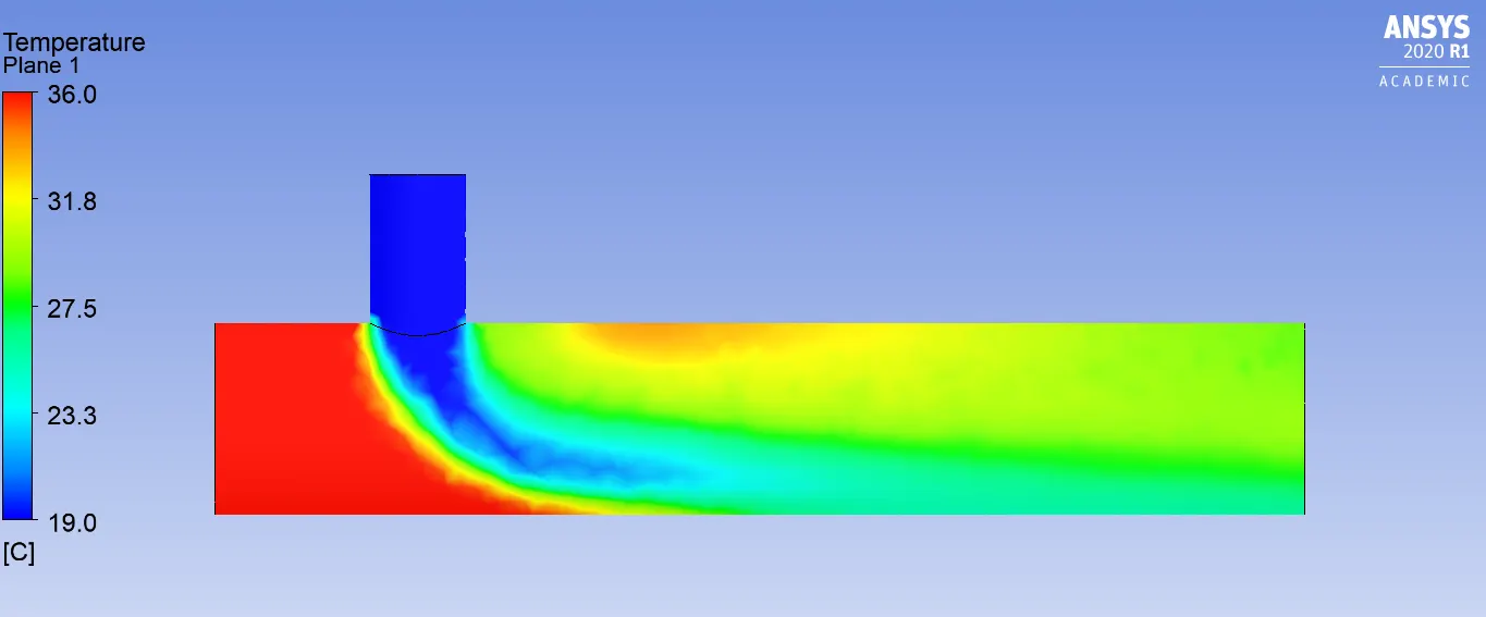
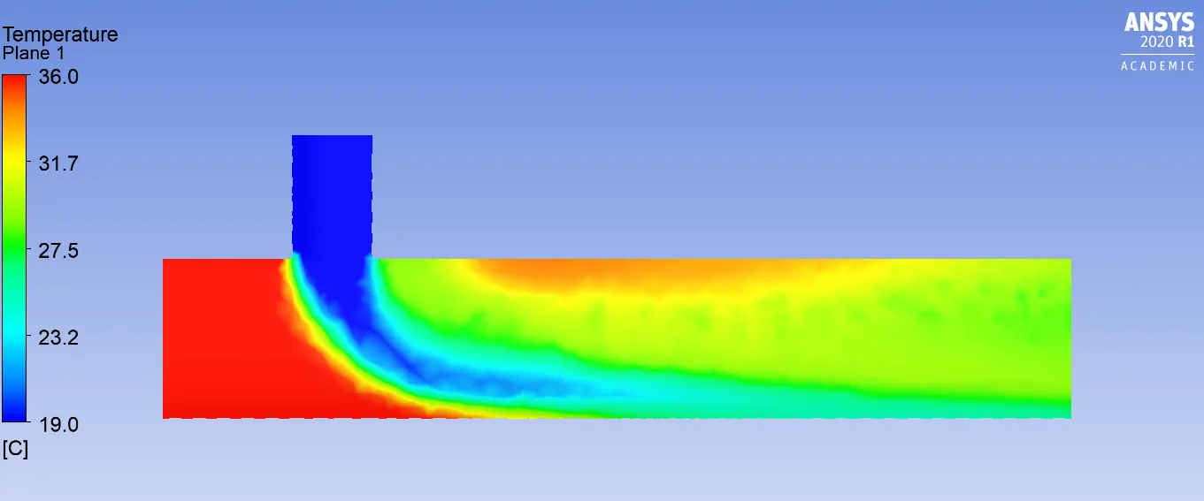
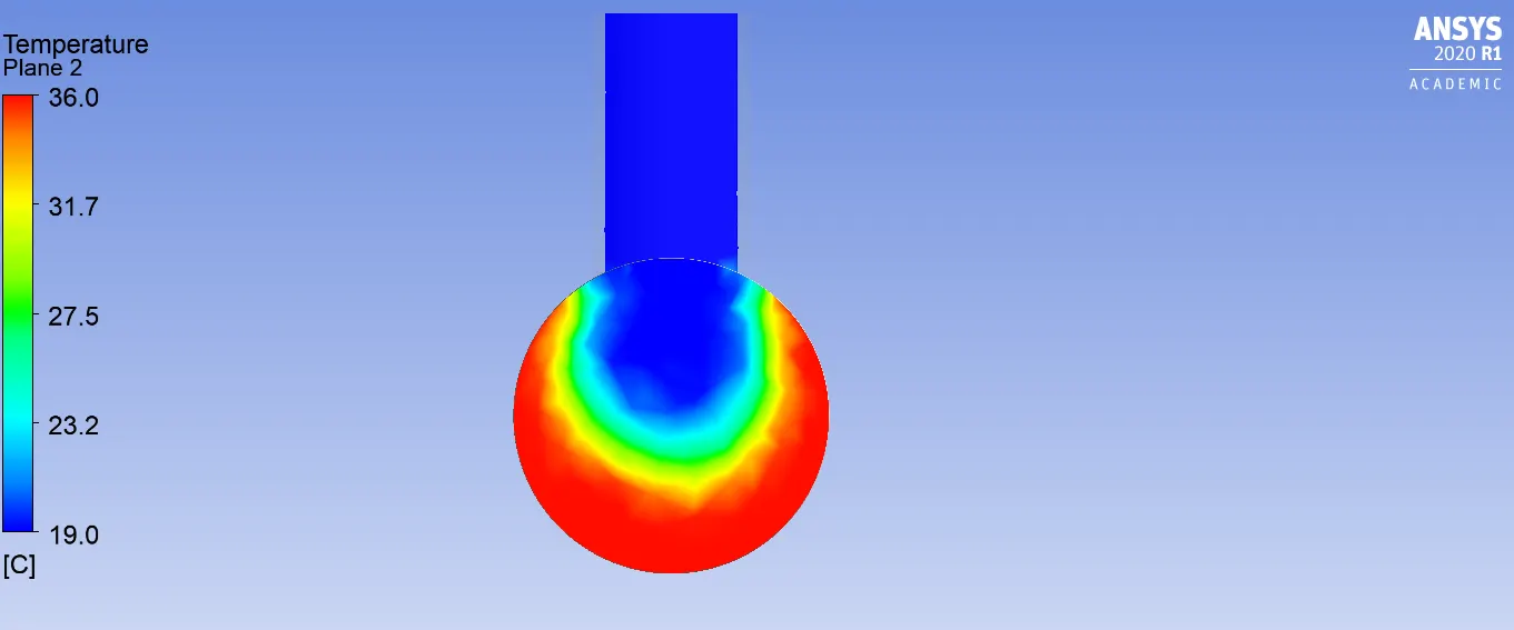
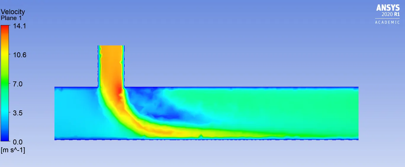
• To plot velocity and temperature contour on the cut planes along and across pipes.
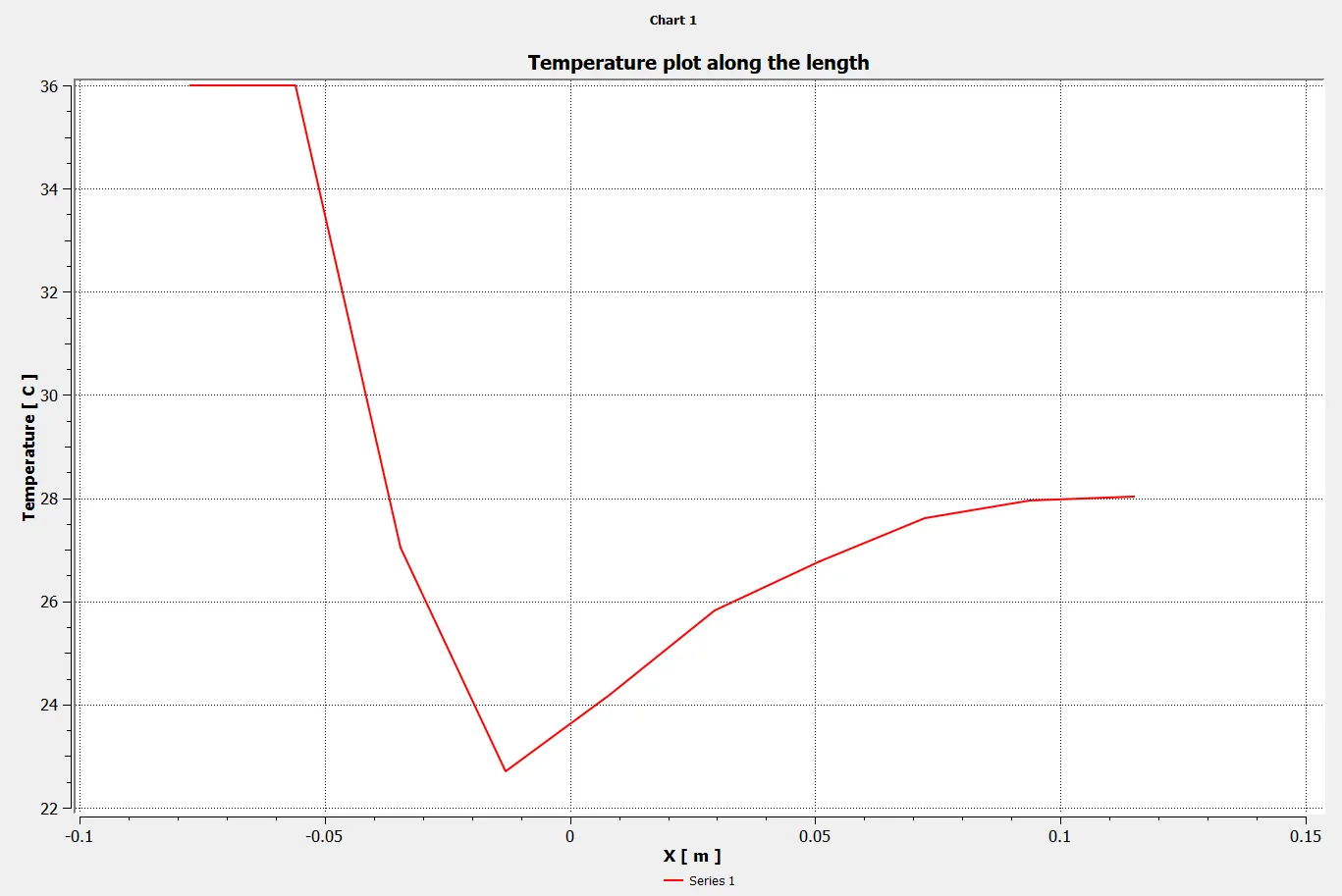
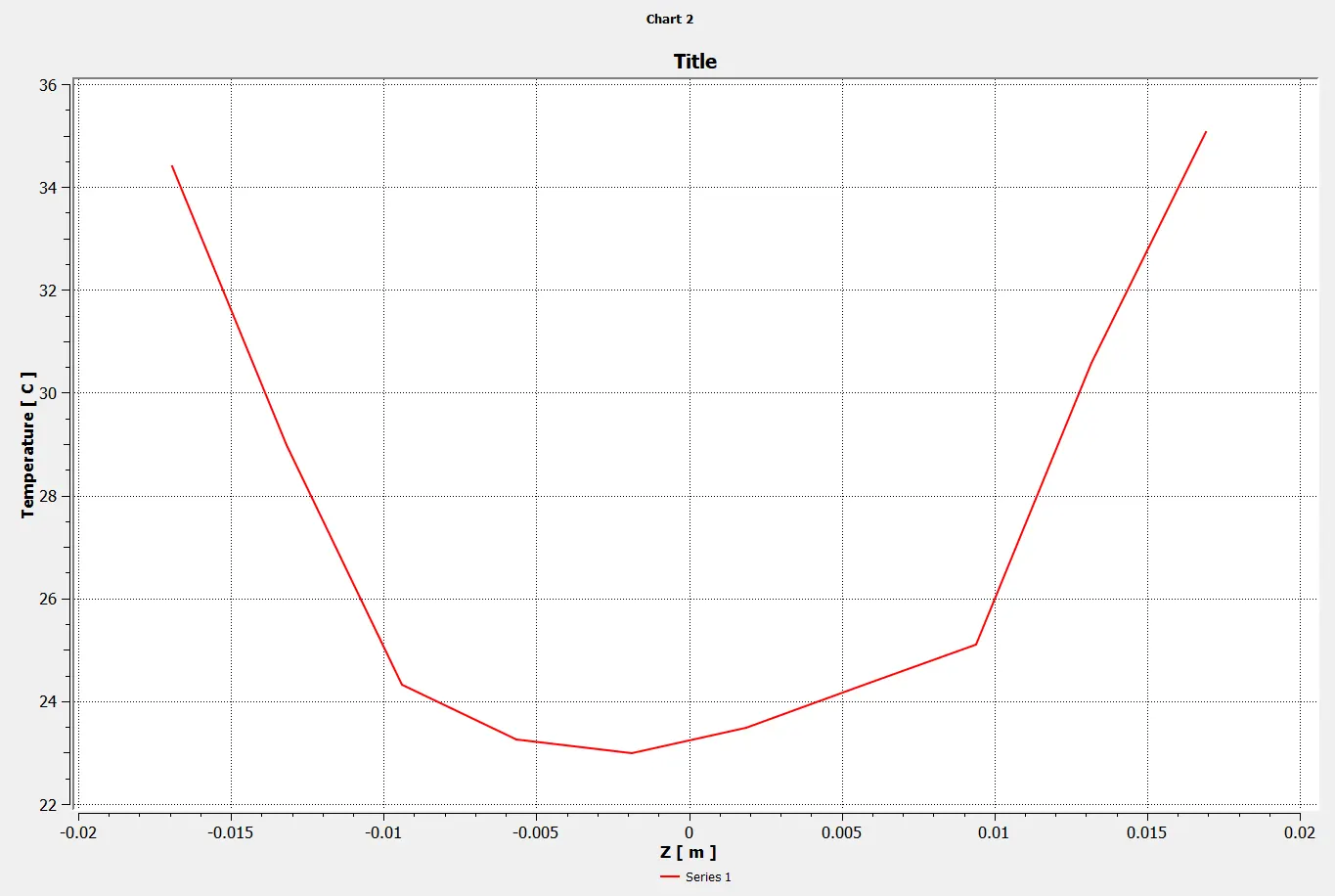
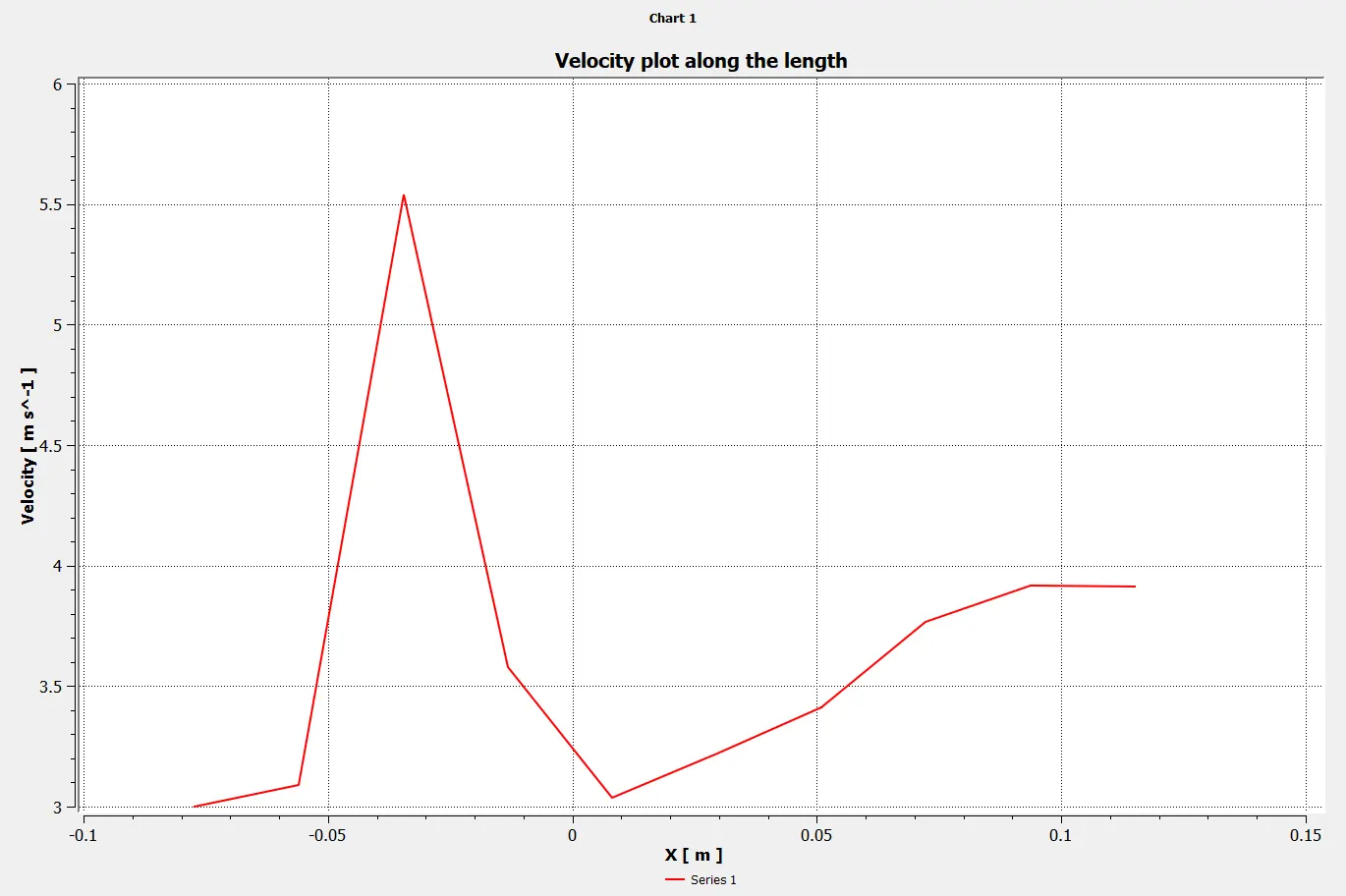
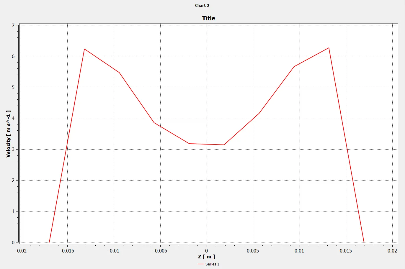
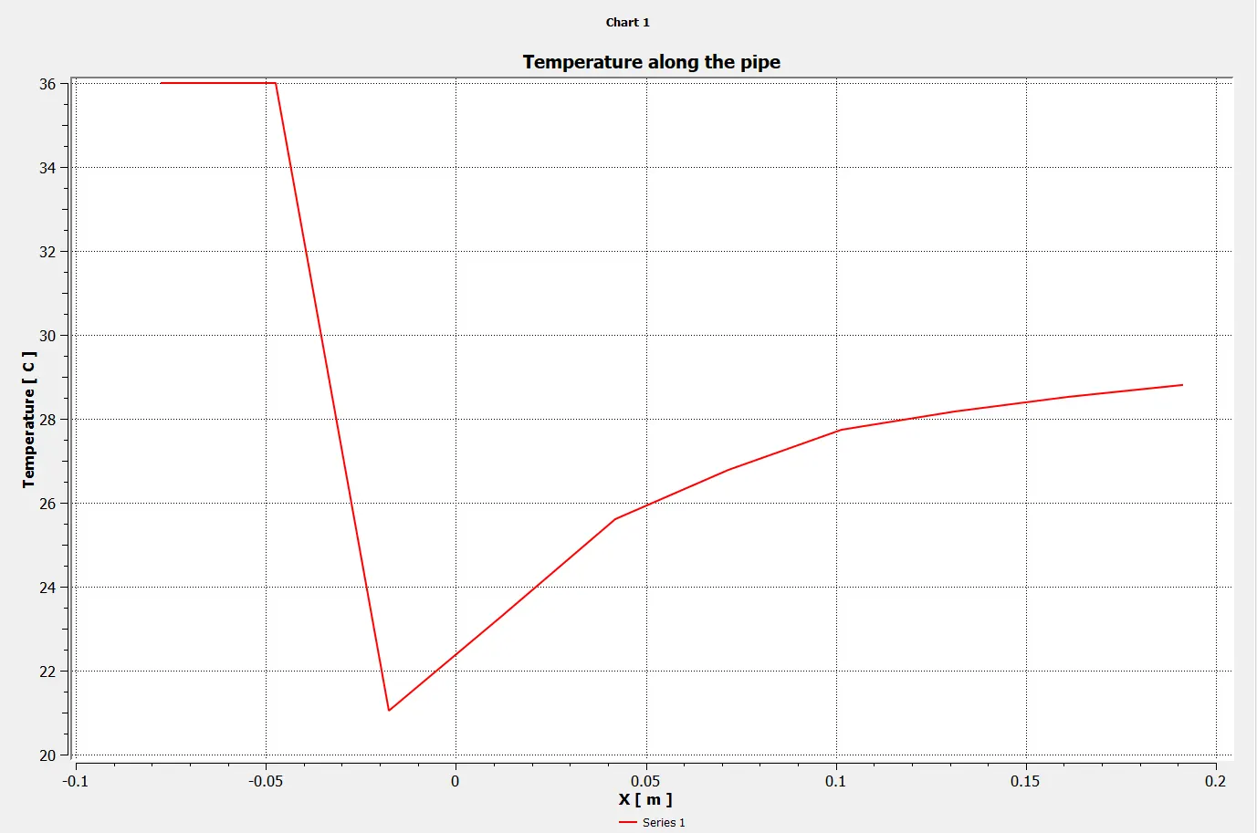
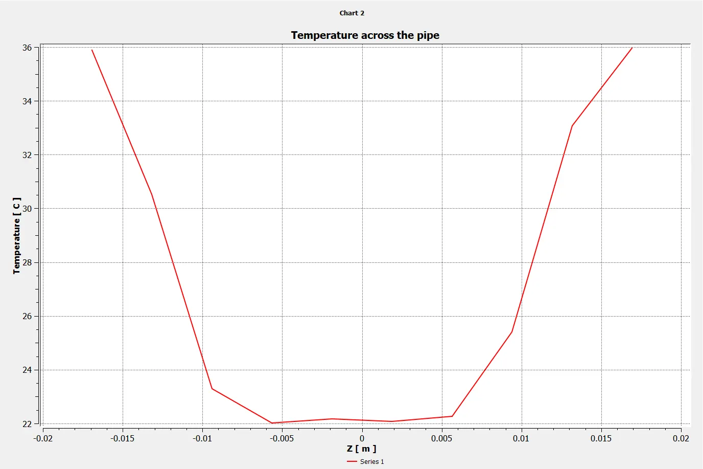
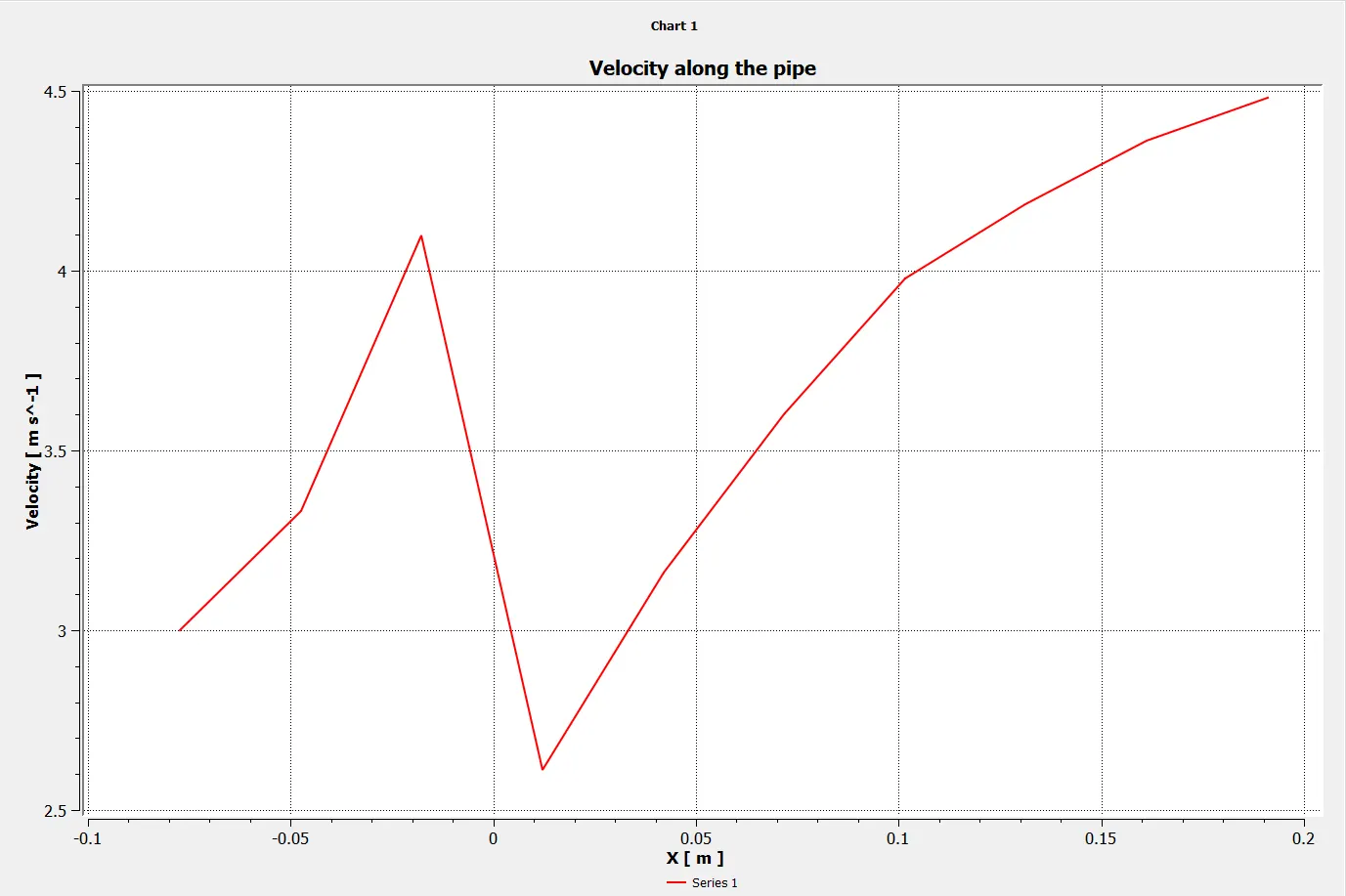
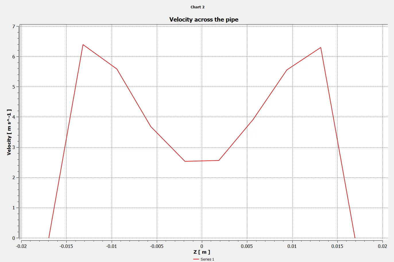
• To plot velocity and temperature line along and across the length of the pipe.
• To perform mesh independent study for any one case.
• To discuss the effect of length and momentum ratio on results.

INTRODUCTION:

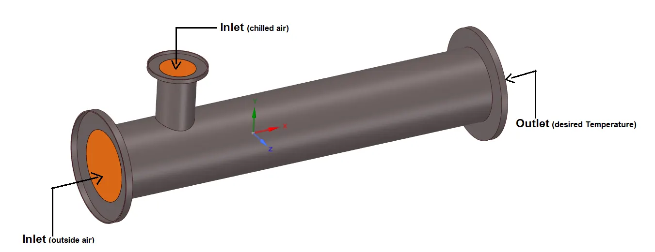
In this project, we are simulating the flow through a short and long tee to measure the mixing effectiveness.In this model the outside air comes through one of the inlet and cold air comes through the other inlet.By adjusting the flowrate of cold air we can get the dezired temperature at the outlet.Here,we will be using K-epsilon and k-omega SST turbulence models which are basically known as RANS MODELS.

THEORY:

Mixing tee joint:-Tee joint are important flow control devices it is T-shaped joint because it splits the flow and angle between them is 90°.It has two inlets and one outlet,it is used in various conditions and various circumstances.Mixing tee efficiently mix two fluid streams into one combined stream.

K-Epsilon turbulence model:- It is the most common model used in computational fluid dynamics to simulate mean flow characteristics for turbulent flow conditions.It is a two equation model that gives a general description of turbulence by means of two transport equation.The original impetus for the K-epsilon model was to improve the mixing length model,as well as to find an alternative to algebraically prescribing turbulent length scales in moderate to high complexity flows.

• The first transported variable is the turbulence kinetic energy(K).
• The second transported variable is the rate of dissipation of turbulence kinetic energy.

K-Omega turbulence model:- It is a common two equation turbulence model,that is used as a closure for the Reynolds averaged Navier Stokes equation.The model attempts to predict turbulence by two partial differential equations for two variables.

• The first variable is turbulent kinetic energy(K).
• The second variable is the specific rate of dissipation of turbulence kinetic energy into internal thermal energy.

PROCEDURE:

---->>>CASE 1:-

Geometry:

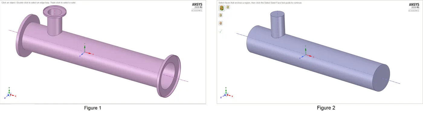
• The below figure 1 is the actual CAD solid model of the Short mixing tee joint with two inlets and one outlet.It includes flow volume and unnecessary geometry that we don't require for the flow simulation.This model is uploaded to Ansys Spaceclaim using step file format.
• Now we need to eliminate the unnecessary geometry using volume extract tool in Ansys Spaceclaim,the fluid volume can be extracted from the model for the simulations as shown in the below figure 2.

Meshing:

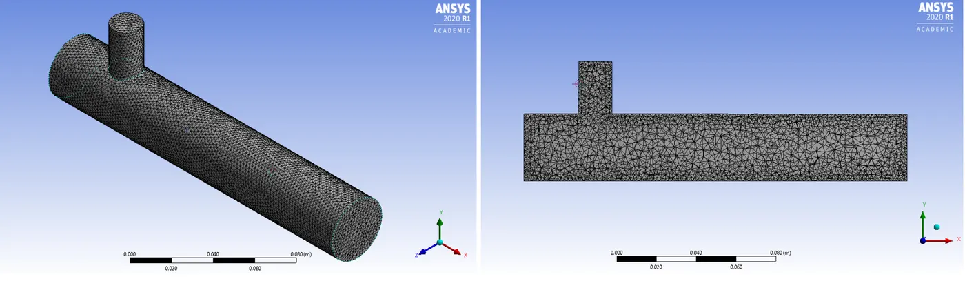
Here we need to name the boundaries we have using named selection option as inlet_x,inlet_y,outlet and wall.Then,we need to put appropriate mesh for a model using generate mesh option.

Element size	2mm
Number of Nodes	21347
Number of Elements	105865

Mesh quality:

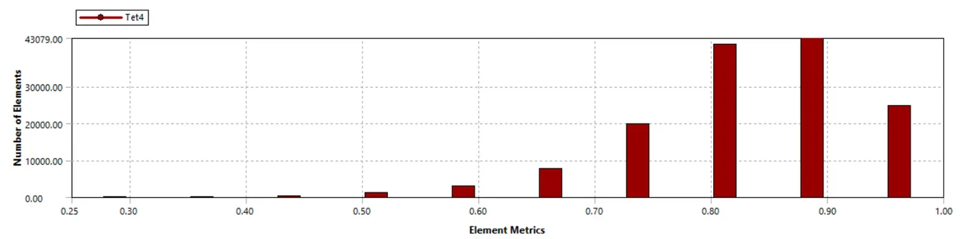
We can check the quality of the mesh by Mesh Metric option in the quality section.The below histogram shows the quality of the mesh by comparing Element matrices to Number of elements.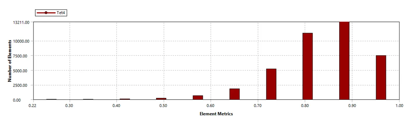

Setup:

1) K-Epsilon Model:-

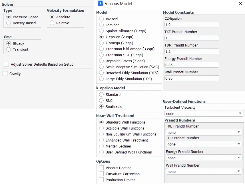
• Here, we need to setup a solver.The solver type is pressure based,steady state condition and we need to select Absolute velocity formation.
• After the solver setup,In the physics we need to select energy option and in viscous model select K-Epsilon model.K-Epsilon is suitable for high reynolds number or in other word it is good for simulation of free flow.

Boundary Conditions:

• After selecting viscous model we need to assaign the boundary conditions to the different parts of the model.Since, we have already assigned the proper name for the boundaries, it automatically selects the boundary conditions.For inlet_x and inlet_y it should be velocity inlet,for outlet it should be pressure outlet and for walls it should be wall.Then in edit option we can feed the given temperatures and inlet velocity.
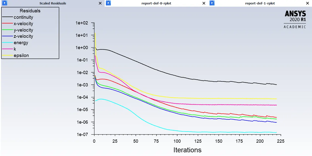
• Then we need to initialize the solver with hybrid scheme and setup number of interations and the click on calculate option.
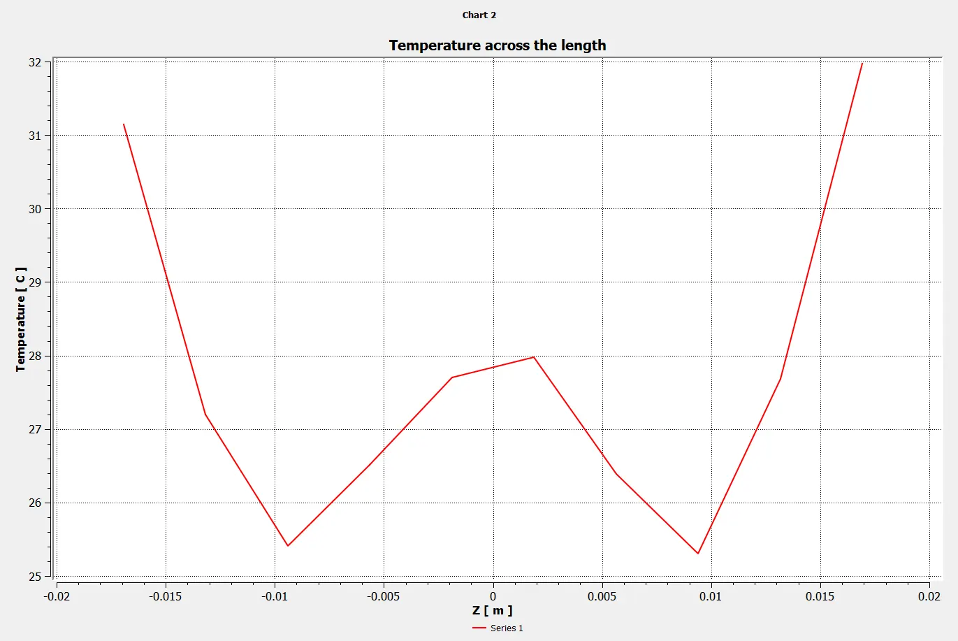
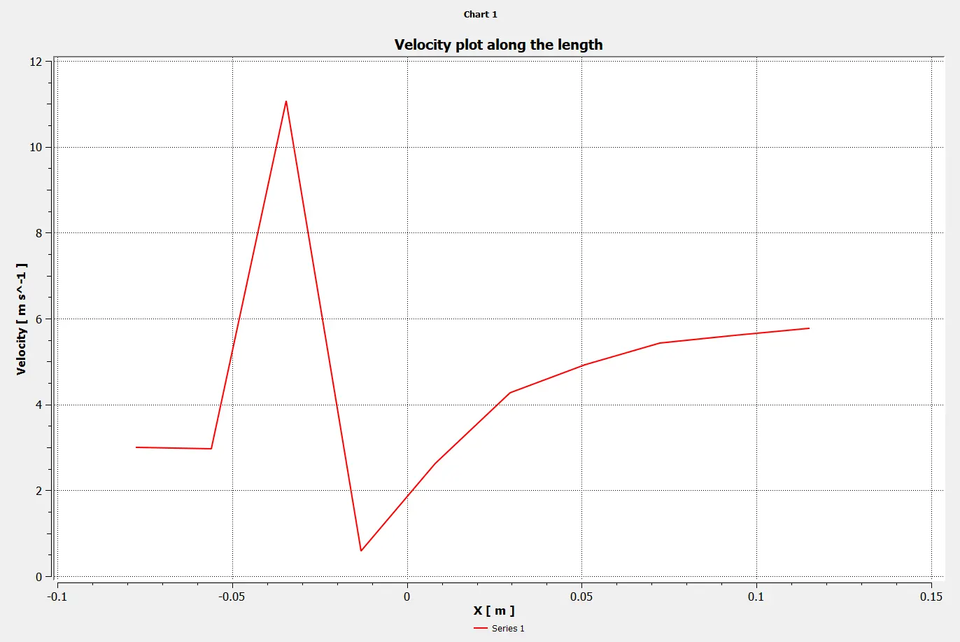
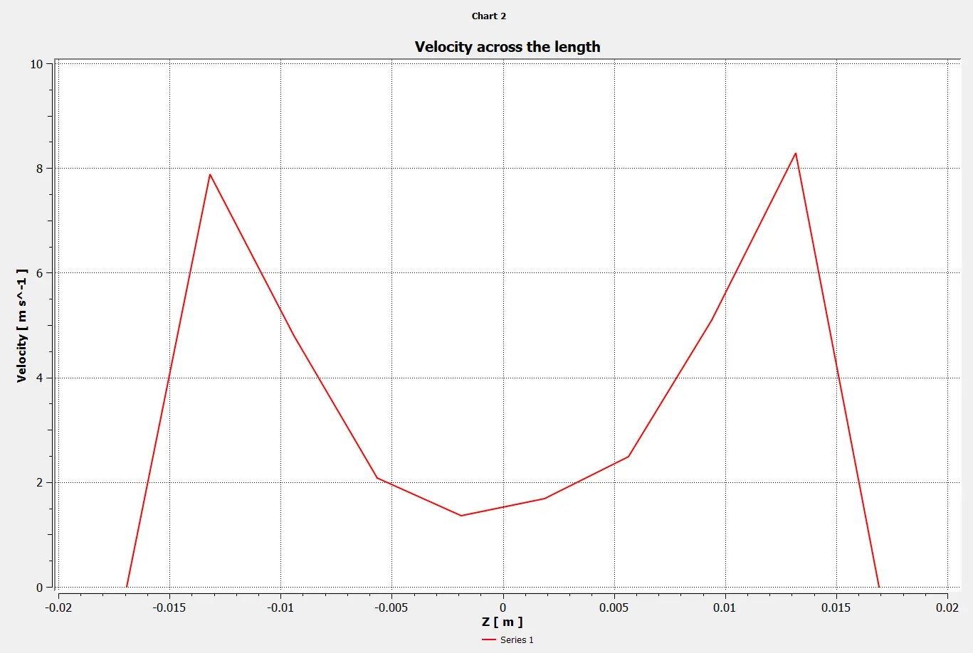
• Then in post processing we need to add a plane and line along and across the pipe, Here we can plot temperature and velocity contour plots and line plots.

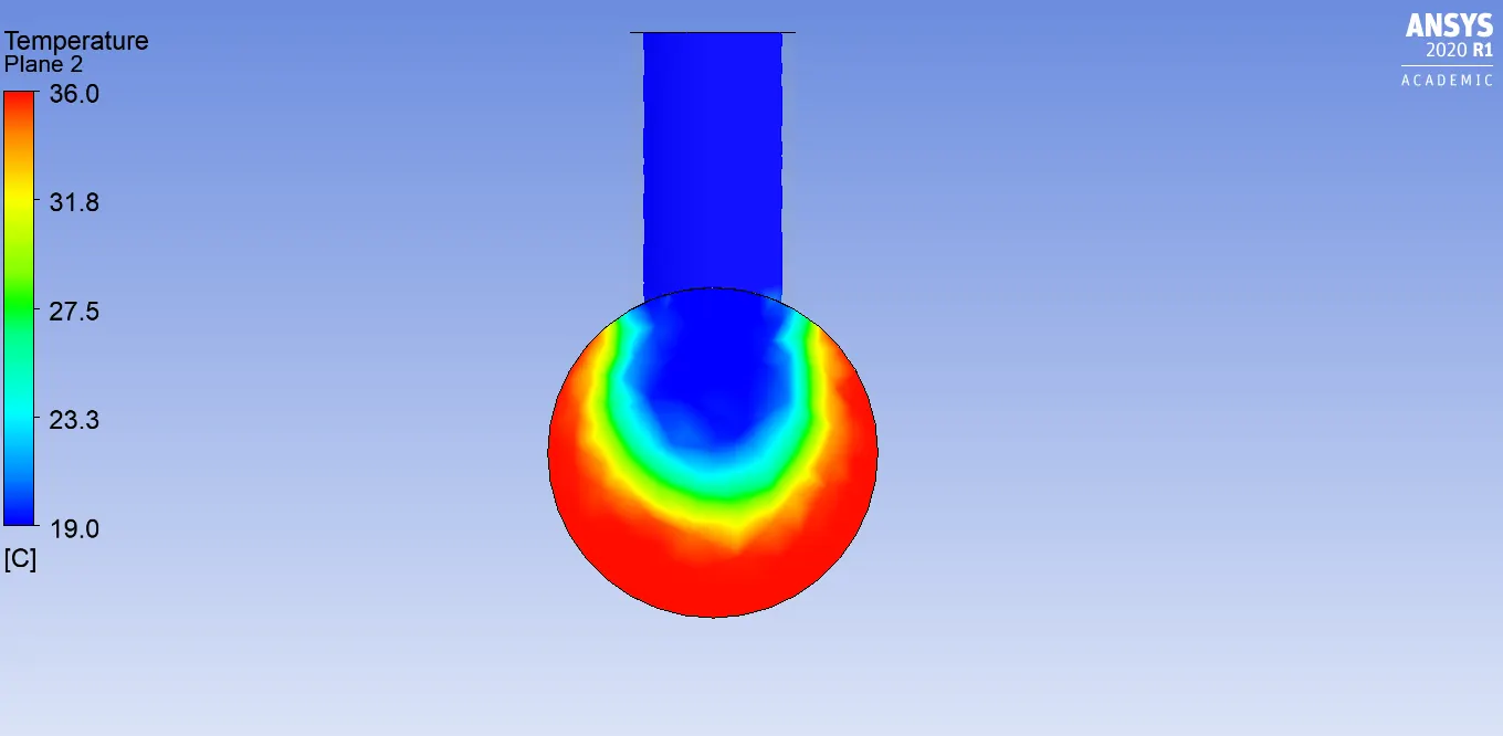
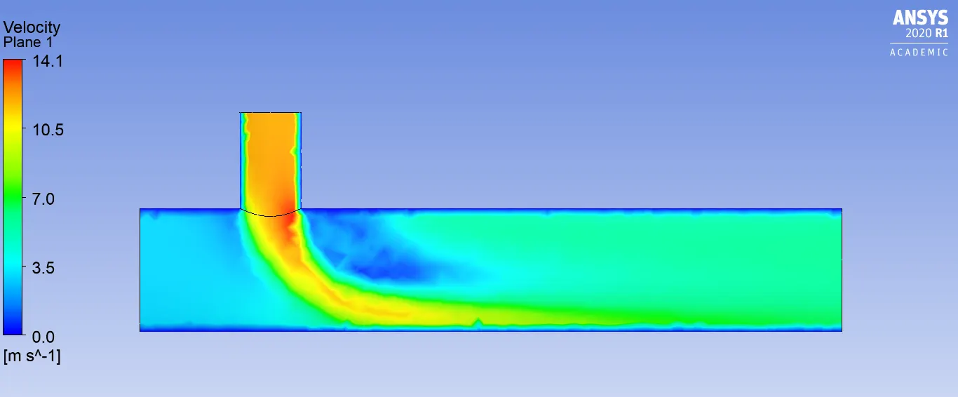
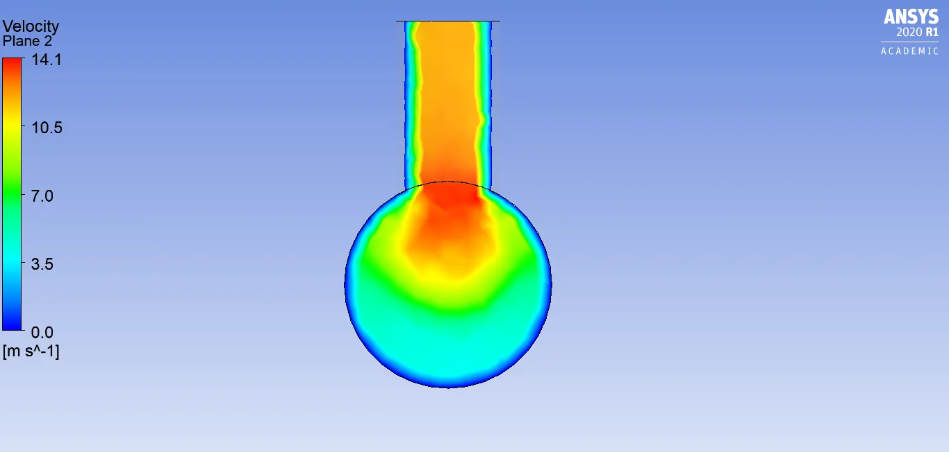
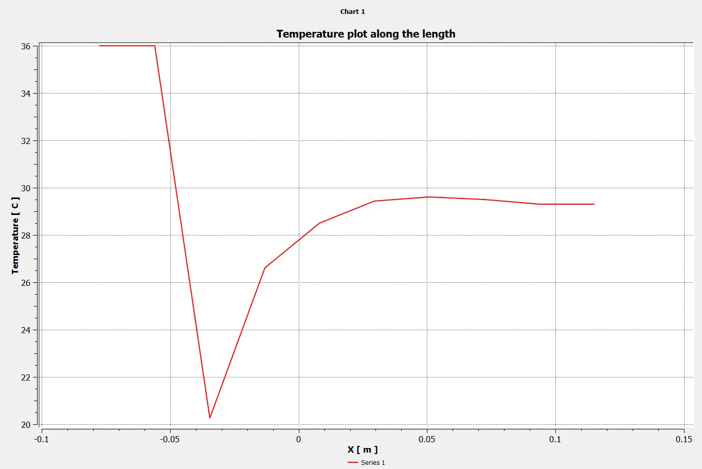
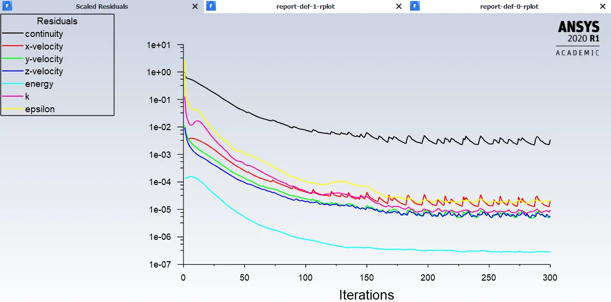
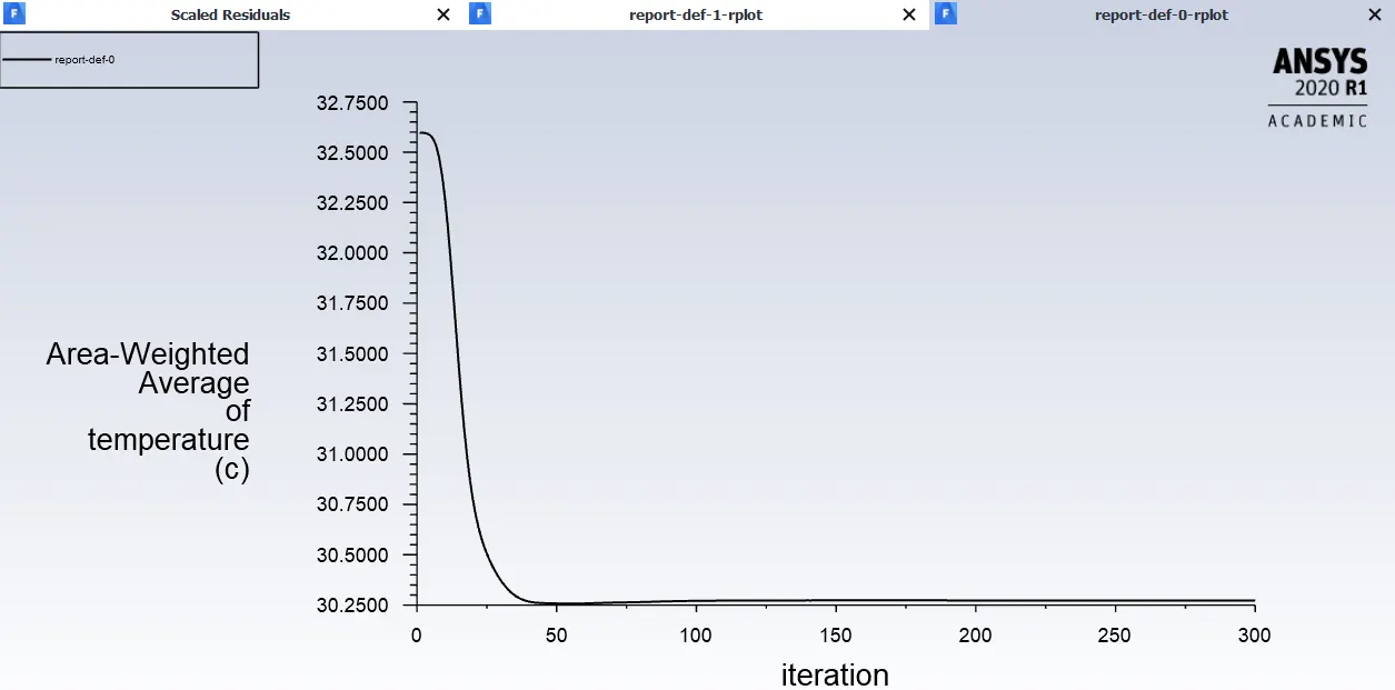
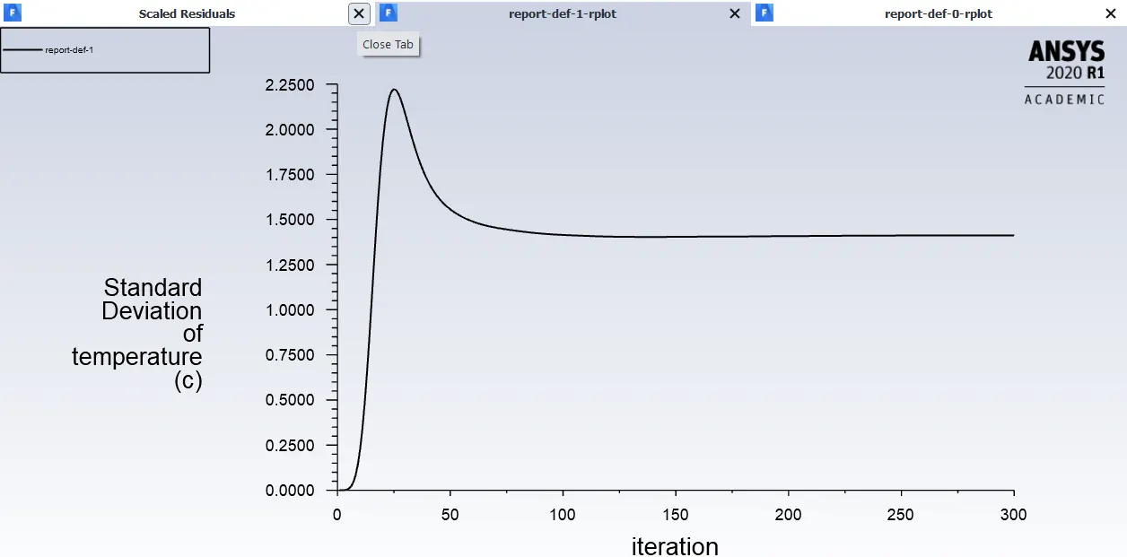
For Momentum ratio=2 Hot inlet Temperature-36° Cold inlet Temperature-19° Hot inlet air velocit-3m/s Cold inlet air Velocity-6m/s (i.e Momentum ratio=2) RESULTS:- Residuals plot Area weighted average of Temperature Standard deviation of temperature POST PROCESSING RESULTS:- Temperature contour along the pipe Temperature contour across the pipe Velocity contour along the pipe Velocity contour across the pipe Temperature line plot along the pipe Temperature line plot across the pipe Velocity line plot along the pipe Velocity line plot across the pipe

For Momentum ratio=4 Hot inlet Temperature-36° Cold inlet Temperature-19° Hot inlet air Velocity-3m/s Cold inlet air Velocity-12m/s (i.e Momentum ratio=4) RESULTS:- Residuals plot Area weighted average of Temperature Standard deviation of temperature POST PROCESSING RESULTS:- Temperature contour along the pipe Temperature contour across the pipe Velocity contour along the pipe Velocity contour across the pipe Temperature line plot along the pipe Temperature line plot across the pipe Velocity line plot along the pipe Velocity line pot across the pipe

2) K-Omega SST model

• After the results and post processing of K-Epsilon model,we need to calculate the results and post processing of K-Omega SST model.
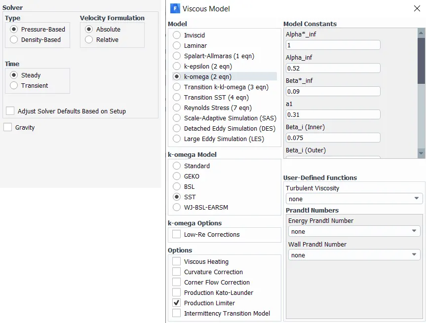
• After the solver setup,In the physics we need to select energy option and in viscous model select K-Omega SST model.

Boundary Conditions

• After selecting viscous model we need to assaign the boundary conditions to the different parts of the model.Since, we have already assigned the proper name for the boundaries, it automatically selects the boundary conditions.For inlet_x and inlet_y it should be velocity inlet,for outlet it should be pressure outlet and for walls it should be wall.Then in edit option we can feed the given temperatures and inlet velocity.
• Then we need to initialize the solver with hybrid scheme and setup number of interations and the click on calculate option.
• Then in post processing we need to add a plane and line along and across the pipe, Here we can plot temperature and velocity contour plots and line plots.

For Momentum ratio=2 Hot inlet Temperature=36° Cold inlet Temperature=19° Hot inlet air Velocity=3m/s Cold inlet air Velocity=6m/s (i.e Momentum ratio=2) RESULTS:- Residuals plot Area weighted average of temperature Standard deviation of temperature POST PROCESSING RESULTS:- Temperature contour along the pipe Temperature contour across the pipe Velocity contour along the pipe Velocity contour across the pipe Temperature line plot along the pipe Temperture line plot across the pipe Velocity line plot along the pipe Velocity line plot across the pipe

For Momentum ratio=4 Hot inlet Temperature=36° Cold inlet Temperature=19° Hot inlet air Velocity=3m/s Cold inlet air Velocity=12m/s (i.e Momentum ratio=4) RESULTS:- Residuals plot Area weighted average of teamperature Standard deviation of temperature POST PROCESSING RESULTS:- Temperature contour along the pipe Temperature contour across the pipe Velocity contour along the pipe Velocity contour across the pipe Temperature line plot along the pipe Temperature line plot across the pipe Velocity line plot along the pipe Velocity line plot across the pipe

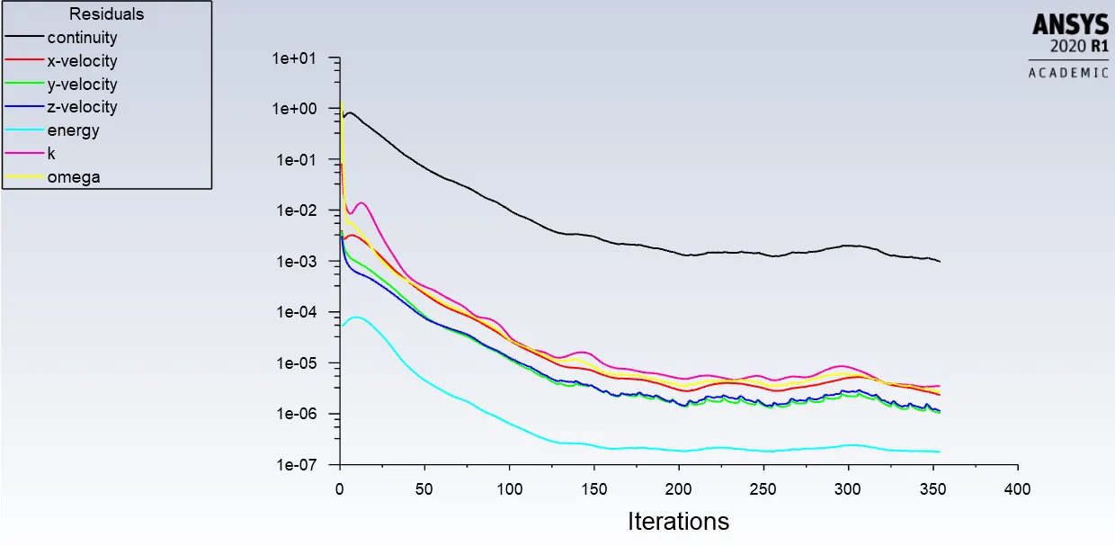
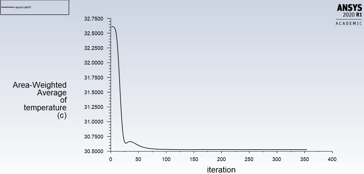
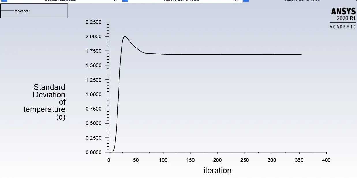
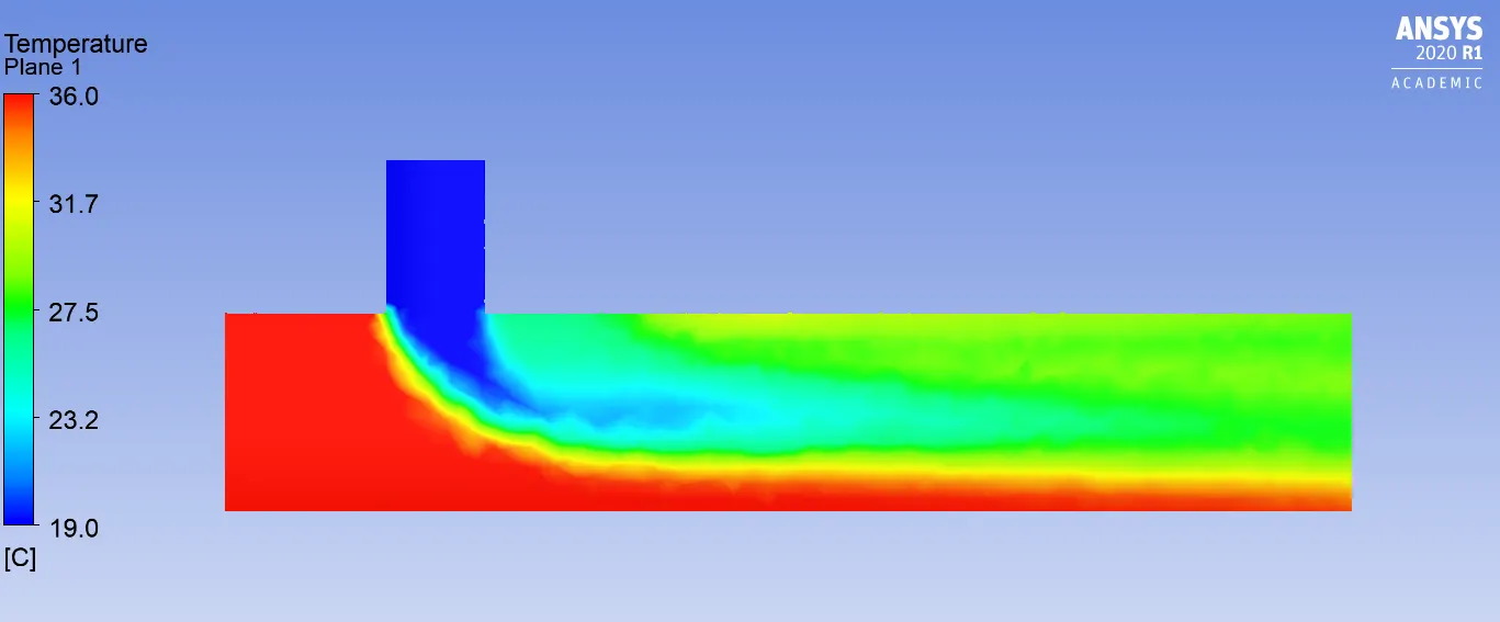
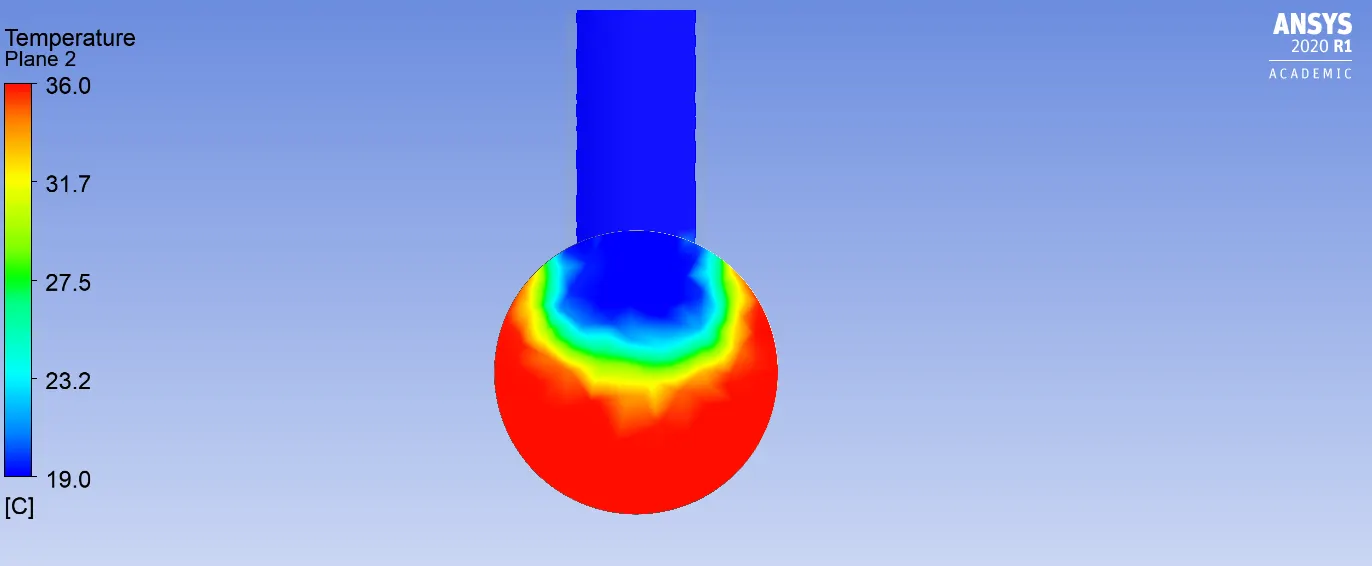
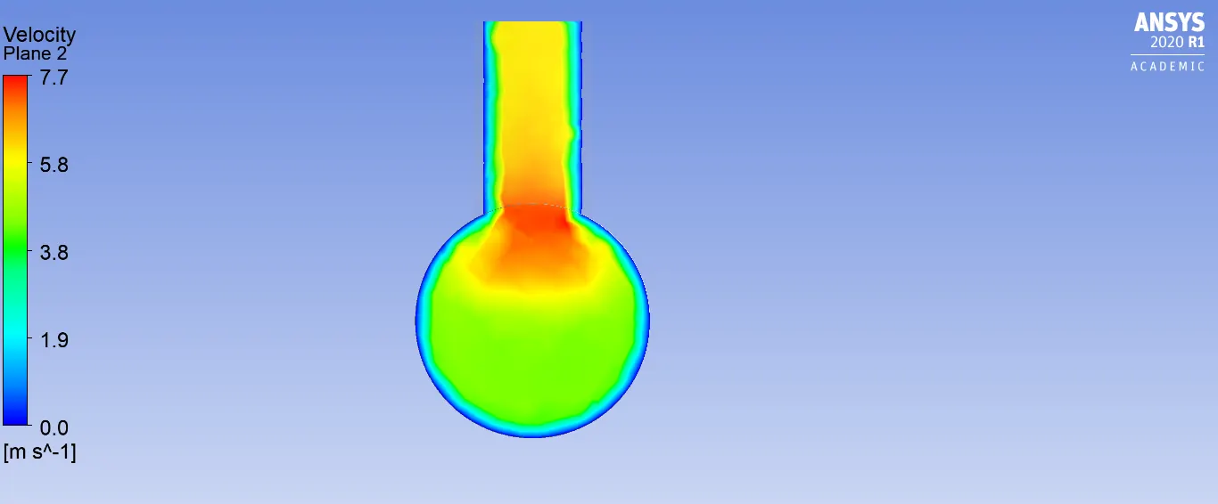
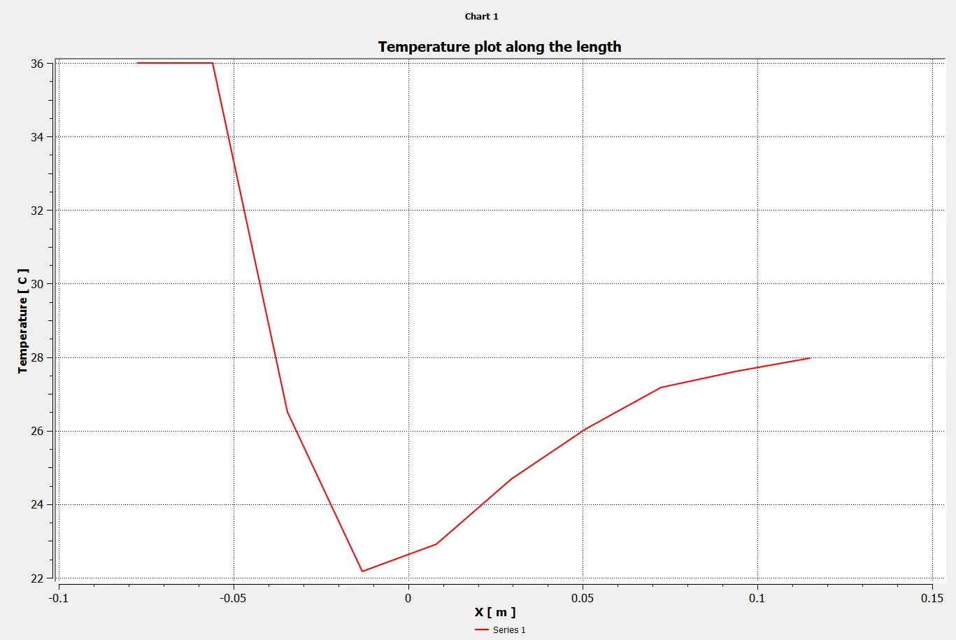
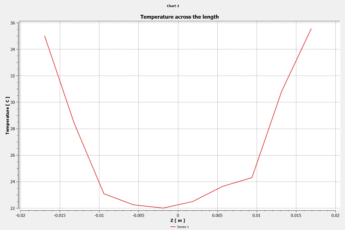
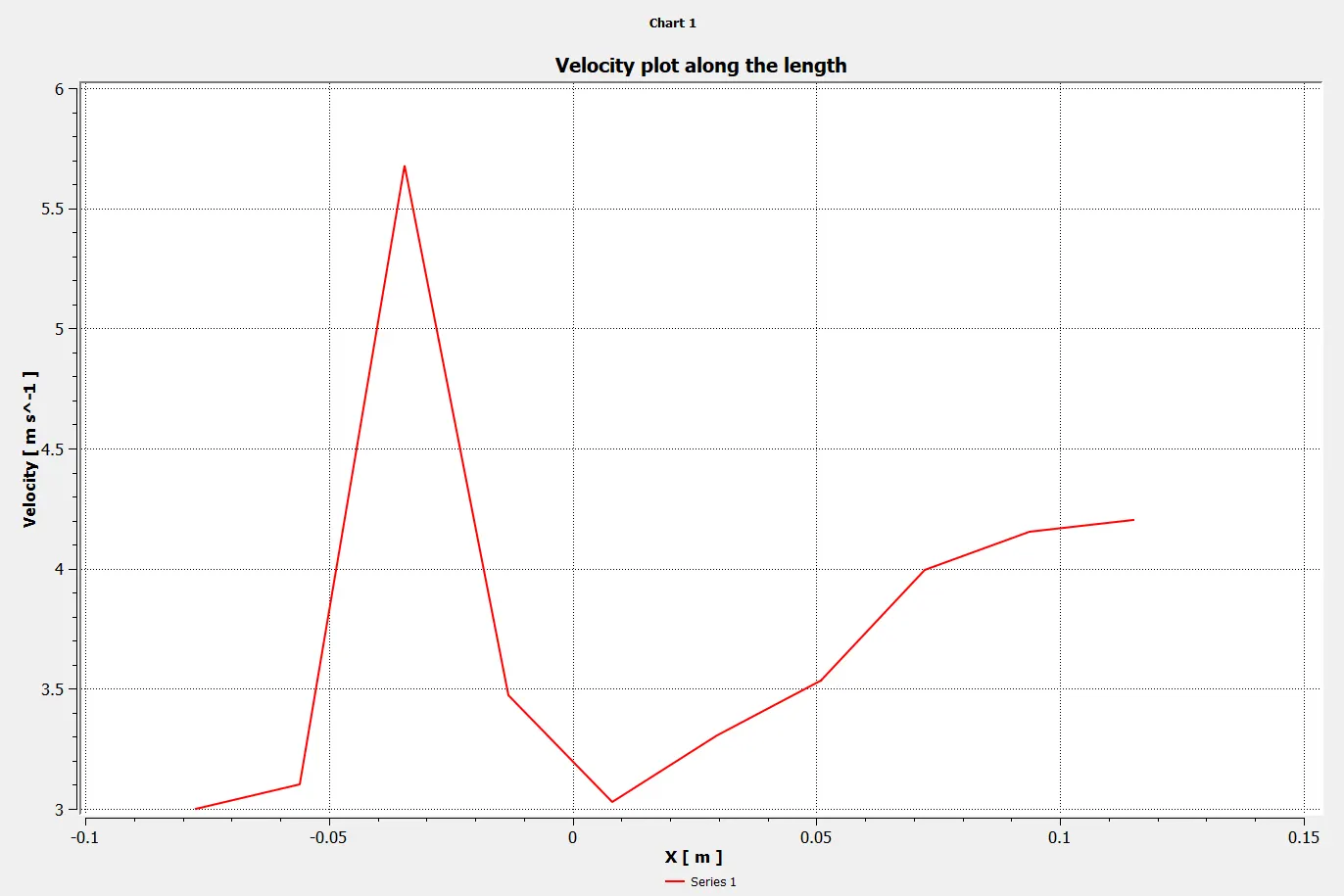
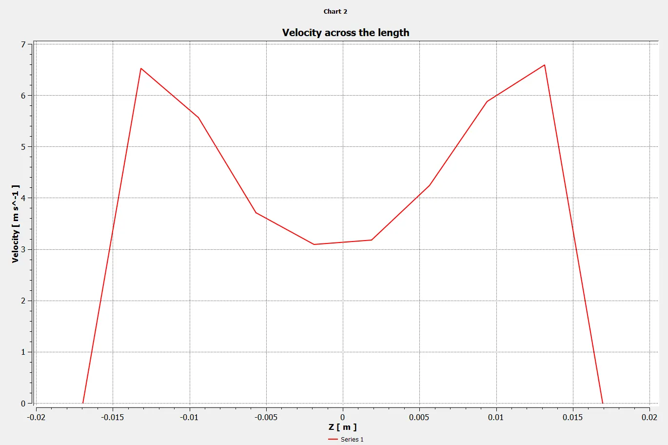
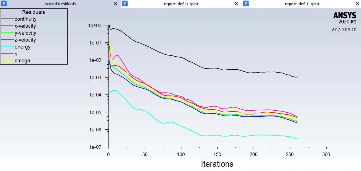
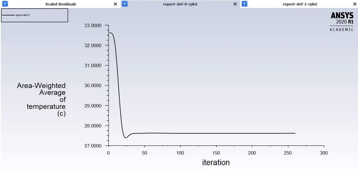
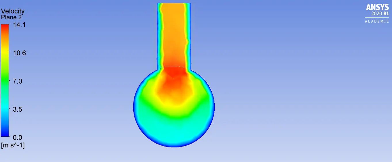
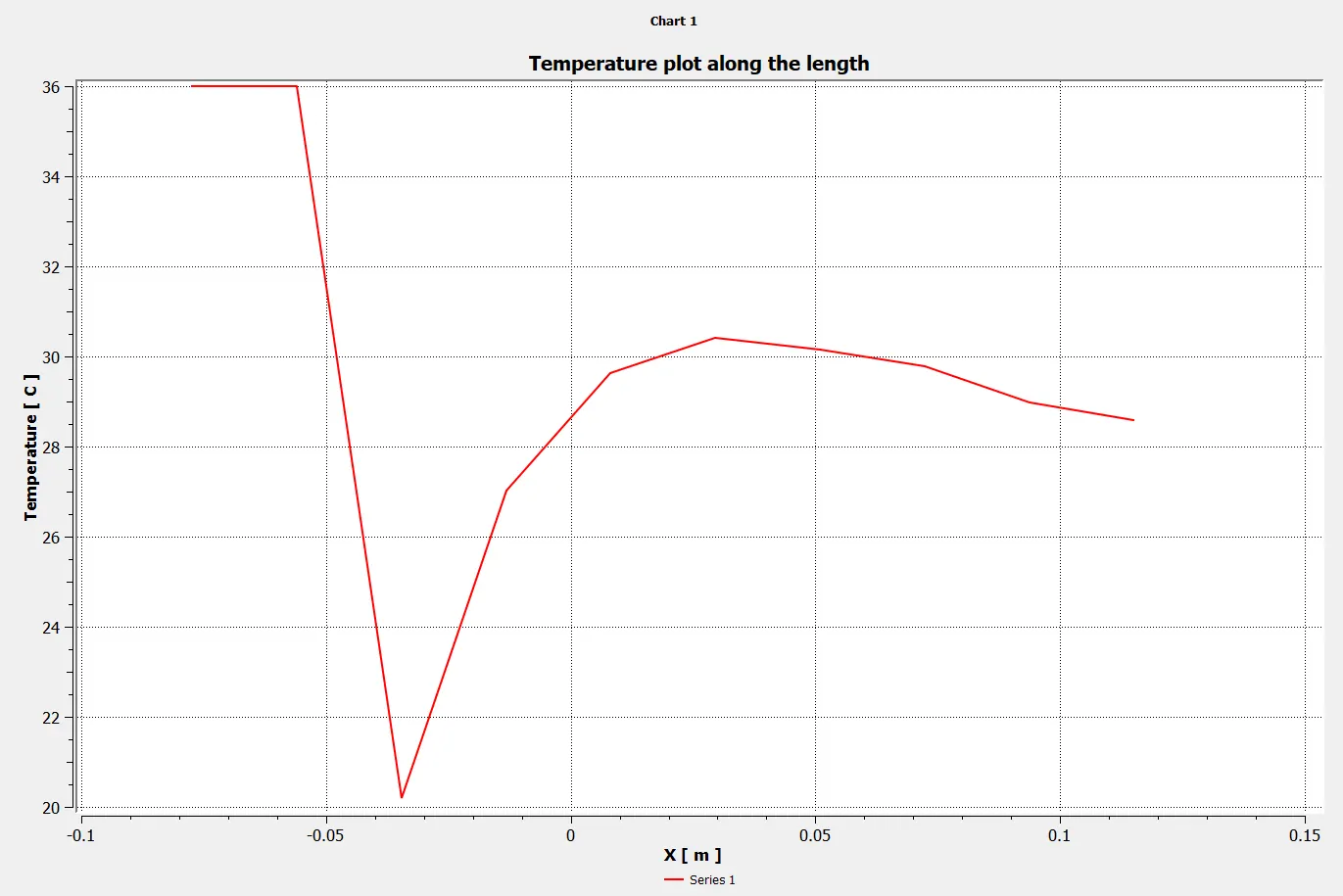
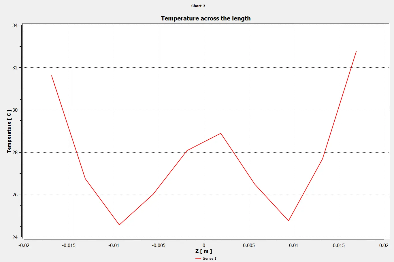
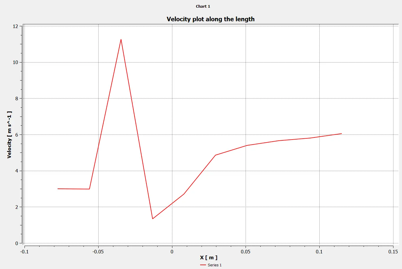
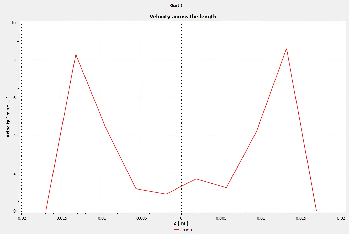
Comparision between K-Epsilon and K-Omega turbulant models for Short tee

Turbulent Model	Momentum ratio	Average outlet Temperature	Standard deviation of Temperature	Iterations to converge
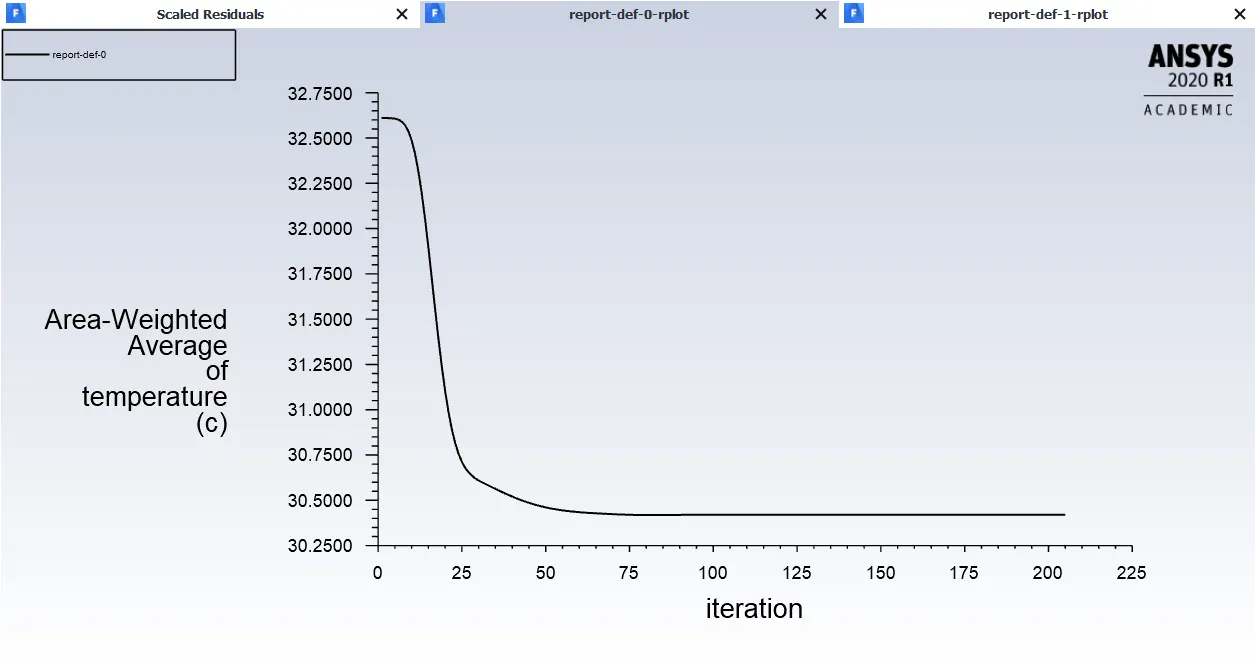
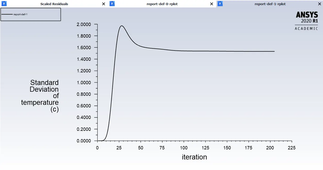
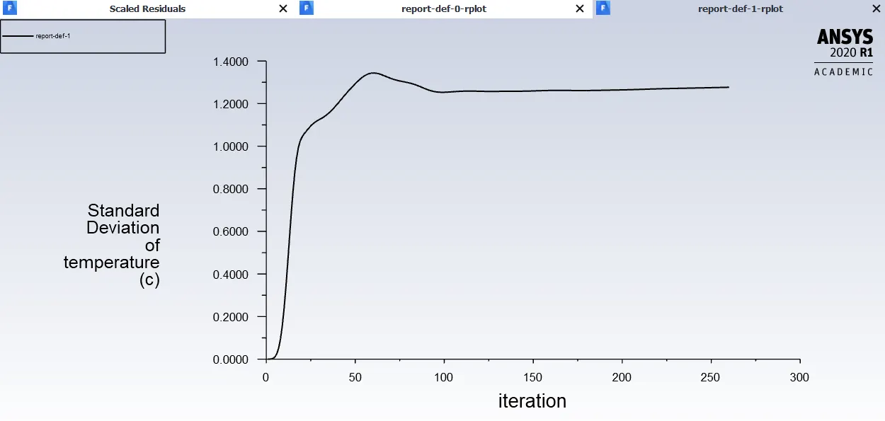
K-Epsilon	2	30.48	1.5	220
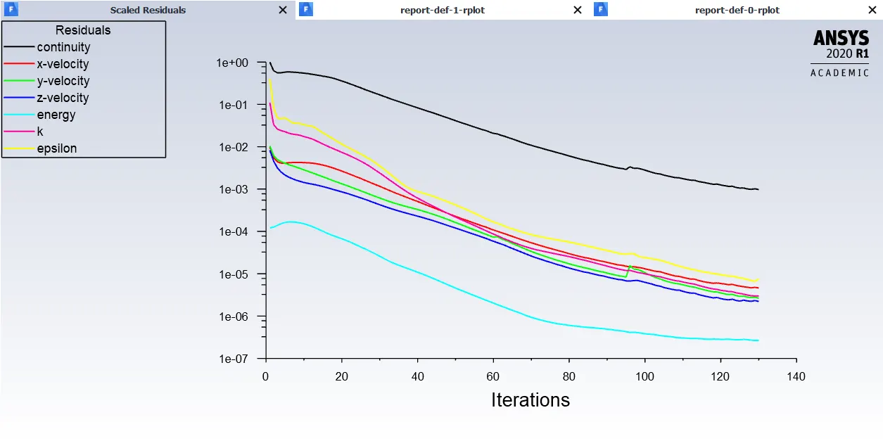
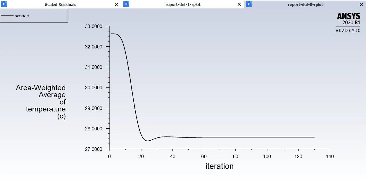
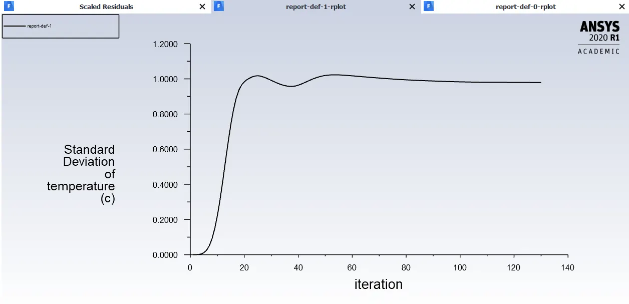
K-Epsilon	4	27.5	0.9	128
K-Omega	2	30.55	1.7	354
K-Omega	4	27.5	1.3	256

Analytical solution:-

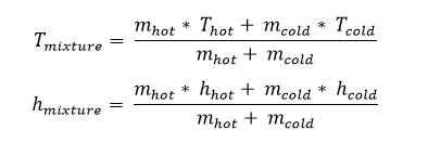
• Density of air= 1.225kg/m^3
• Area of hot air inlet= 0.0009m^2
• Area of cold air inlet= 0.0002m^2
• Velocity of hot air=3m/s
• Temperature of hot air= 36°C --> 309.15K
• Temperature of cold air=19°C --> 292.15K
• Velocity of cold air=6m/s (M.R=2)
• Velocity of cold air= 12m/s (M.R=4)

Momentum ratio=2

• Mass of hot air= 1.225*0.0009*3= 3.3075kg/s
• Mass of cold air=1.225*0.0002*6= 1.47kg/s

• Temperature of mixture = [(3.3075*36)+(1.47*19)] / (3.3075+1.47) = 30.769°C

Momentum ratio=4

• Mass of hot air= 1.225*0.0009*3= 3.3075kg/s
• Mass of cold air= 1.225*0.0002*12= 2.94kg/s

• Temperature of mixture = [(3.3075*36)+(2.94*19)] / (3.3075+2.94) = 28°C

CONCLUSION:-

1) Average outlet temperature for both the turbulent models are almost same.

2) Standard deviation of temperature for K-Epsilon model is lower than K-Omega model.

• Higher the standard deviation lower is the precision and presision is high when standard deviation is low.
• So, K-Epsilon model has high presision than K-Omega model.

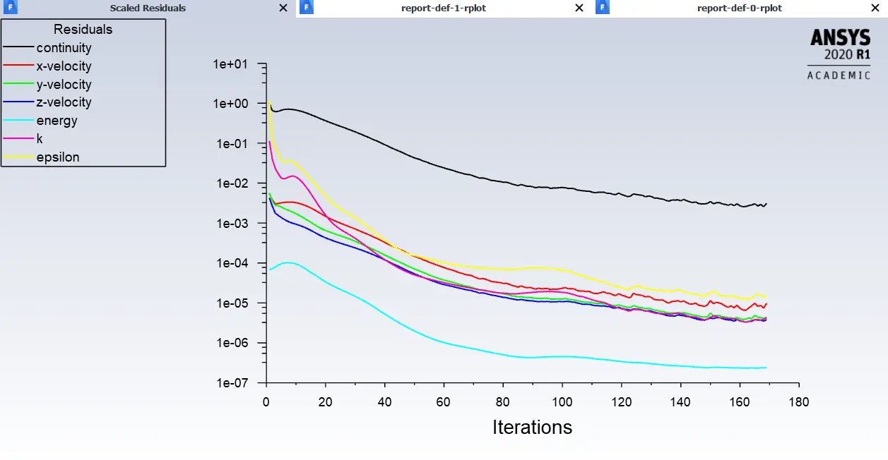
3) Number of iterations taken by K-Epsilon model for convergence is lower than K-Omega model.

• The residual errors are high when number of iterations taken to convergence are more,and residual errors are low if number of iteration taken to convergence are less.
• So, K-Epsilon model has lower residual errors than K-Omega model.

4) K-Epsilon model is used when we need to find the resuts farther to the wall, and K-Omega model is used when we need results near to the wall.

===>From above conclusions we can conclude that K-Epsilon turbulent model is more suitable for mixing tee model because it gives precised results with low residual errors and solution gets converged in less iteratons.

---->>>CASE 2:-

Geometry:

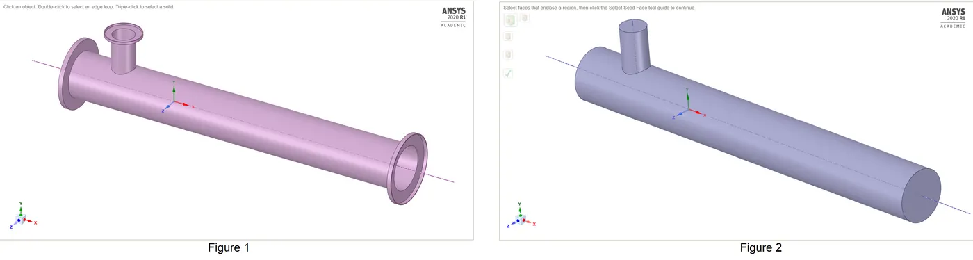
• The below figure 1 is the actual CAD solid model of the Long mixing tee joint with two inlets and one outlet.It includes flow volume and unnecessary geometry that we don't require for the flow simulation.This model is uploaded to Ansys Spaceclaim using step file format.

• Now we need to eliminate the unnecessary geometry using volume extract tool in Ansys Spaceclaim,the fluid volume can be extracted from the model for the simulations as shown in the below figure 2.

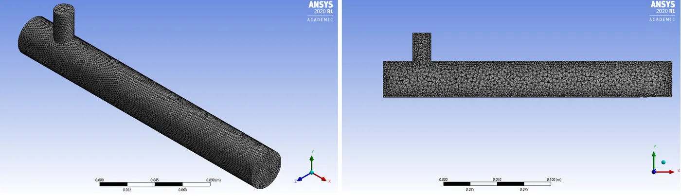
Meshing:

Here we need to name the boundaries we have using named selection option as inlet_x,inlet_y,outlet and wall.Then,we need to put appropriate mesh for a model using generate mesh option.

Element size	2mm
Number of Nodes	28372
Number of Elements	140525

Mesh quality:

We can check the quality of the mesh by Mesh Metric option in the quality section.The below histogram shows the quality of the mesh by comparing Element matrices to Number of elements.

Setup:

1) K-Epsilon Model:-

• Here, we need to setup a solver.The solver type is pressure based,steady state condition and we need to select Absolute velocity formation.
• After the solver setup,In the physics we need to select energy option and in viscous model select K-Epsilon model.K-Epsilon is suitable for high reynolds number or in other word it is good for simulation of free flow.

Boundary Conditions:

• After selecting viscous model we need to assaign the boundary conditions to the different parts of the model.Since, we have already assigned the proper name for the boundaries, it automatically selects the boundary conditions.For inlet_x and inlet_y it should be velocity inlet,for outlet it should be pressure outlet and for walls it should be wall.Then in edit option we can feed the given temperatures and inlet velocity.
• Then we need to initialize the solver with hybrid scheme and setup number of interations and the click on calculate option.
• Then in post processing we need to add a plane and line along and across the pipe, Here we can plot temperature and velocity contour plots and line plots.

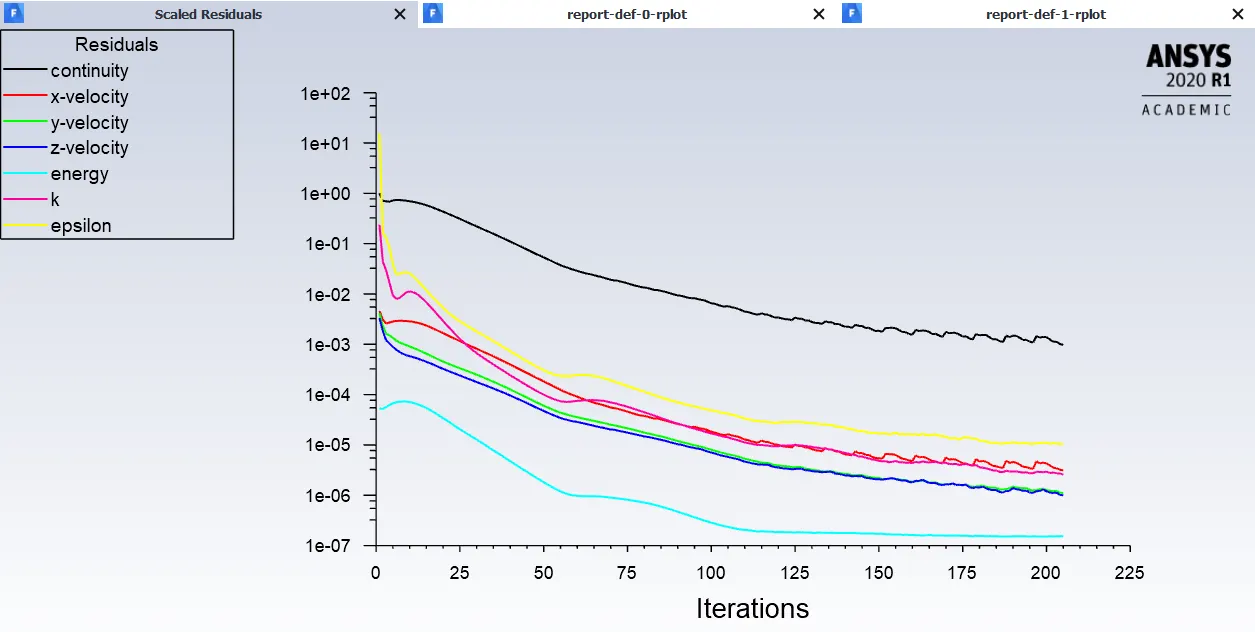
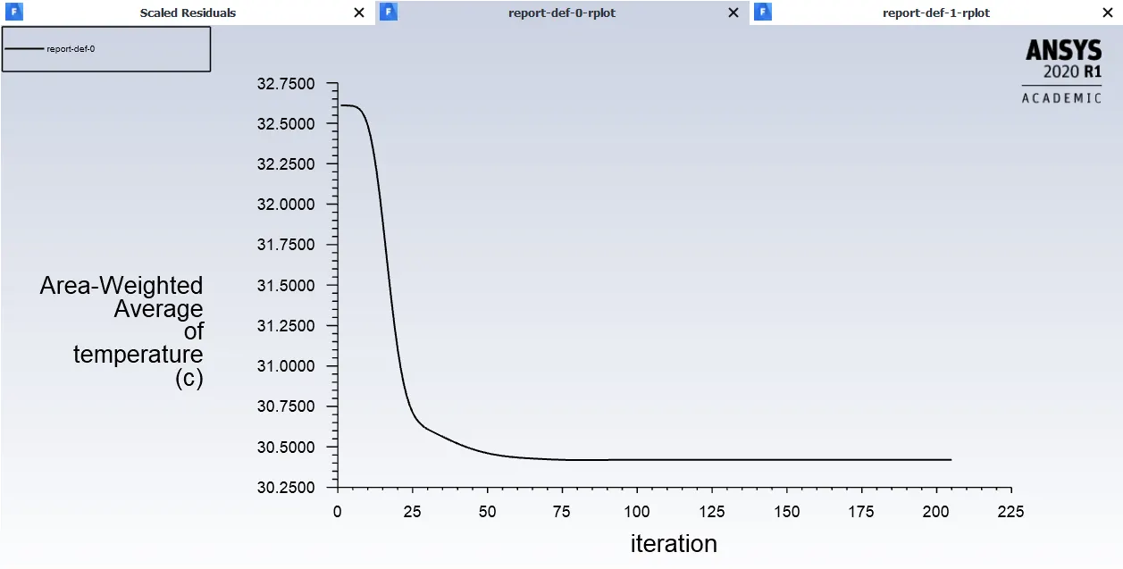
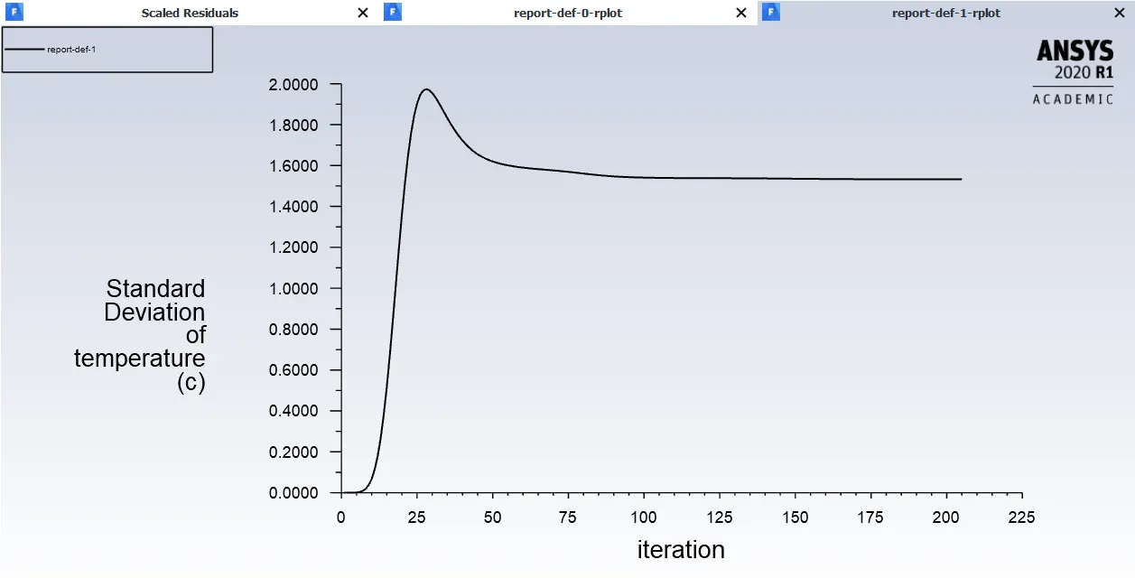
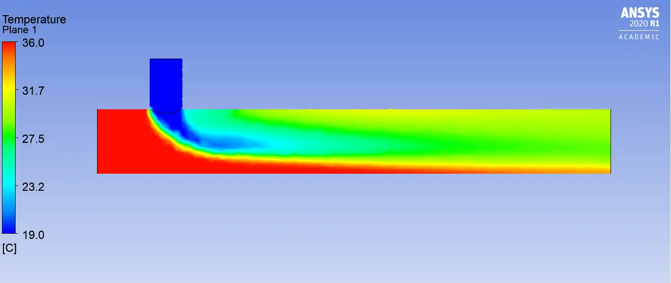
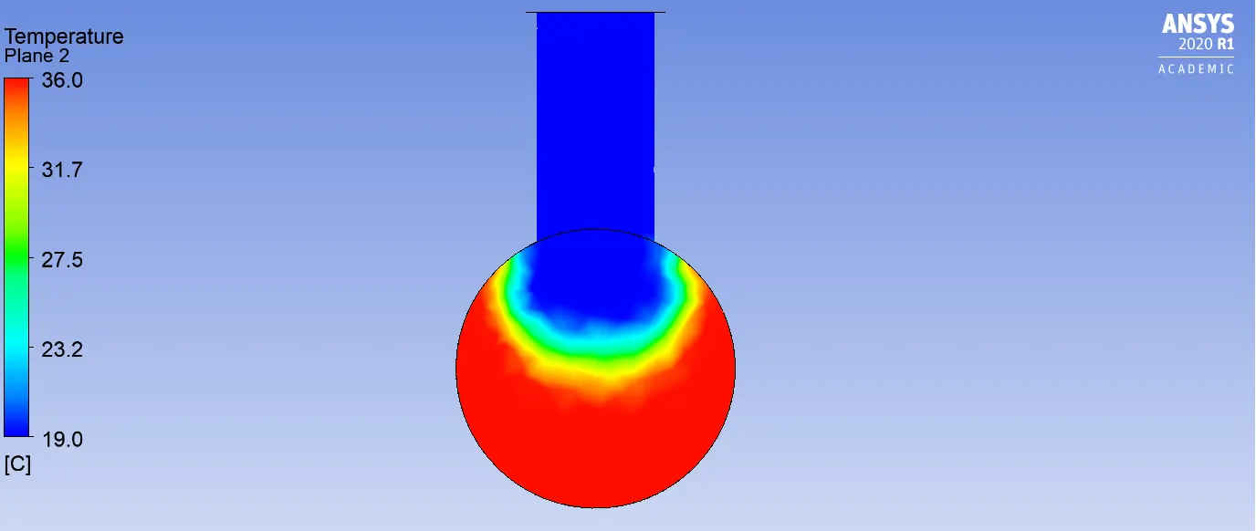
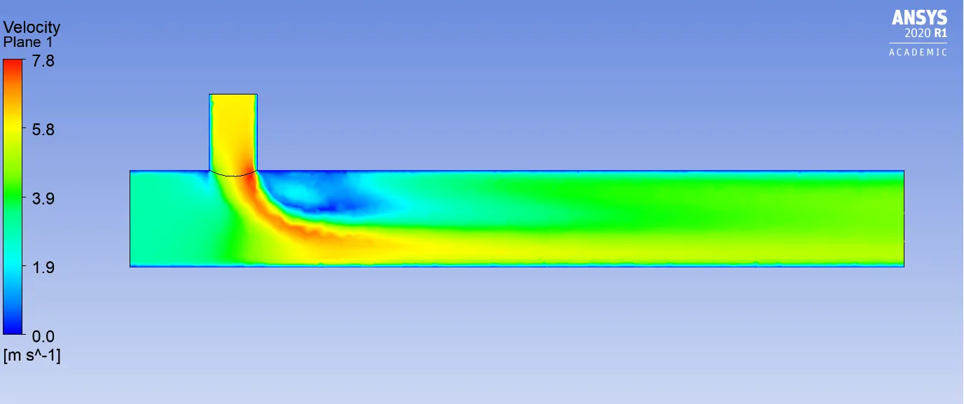
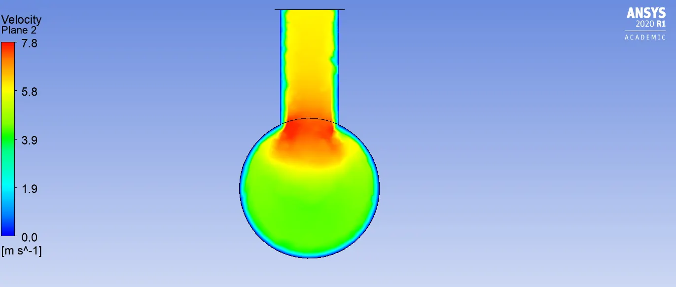
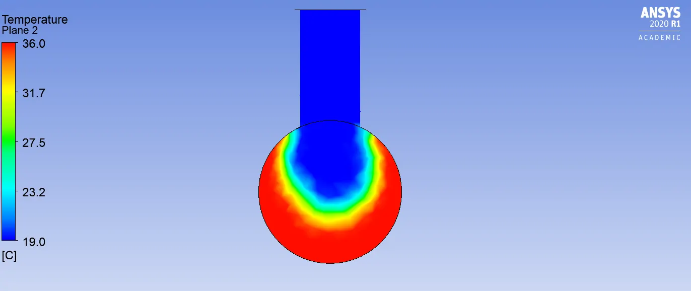
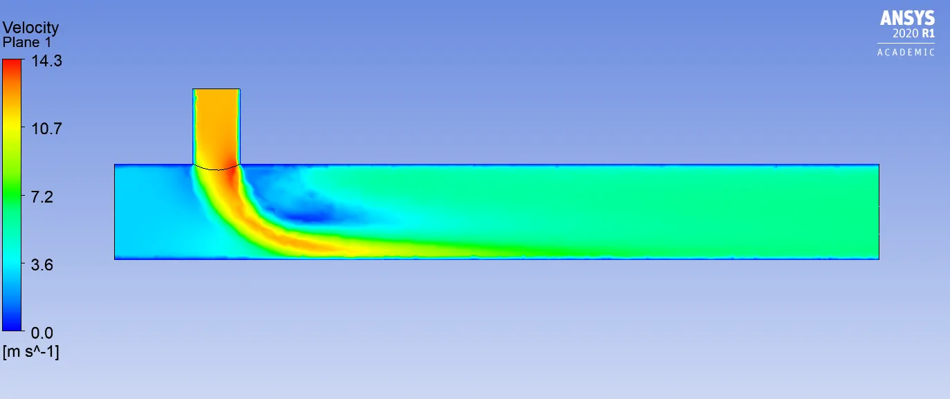
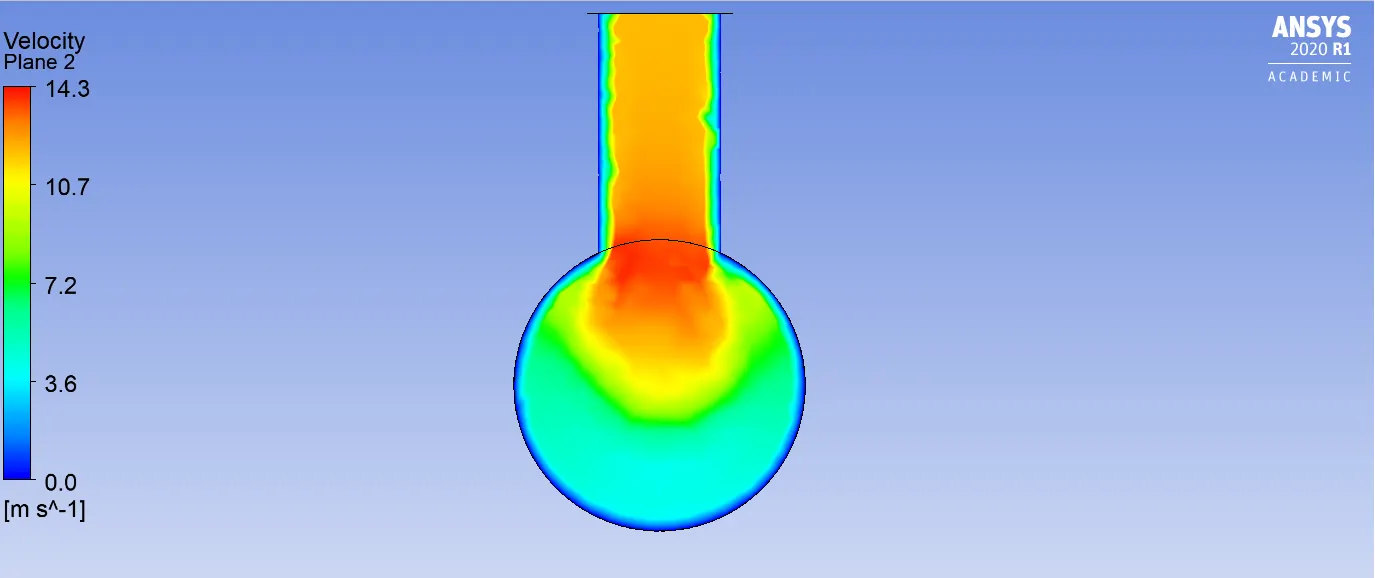
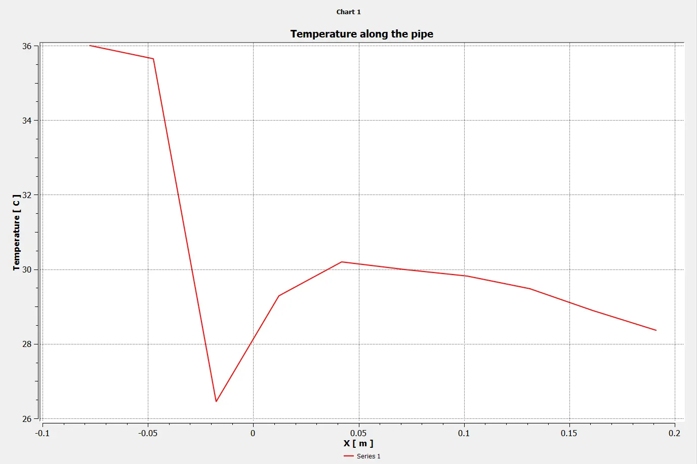
Momentum ratio=2 Hot inlet Temperature=36° Cold inlet Temperature=19° Hot inlet air Velocity=3m/s Cold inlet air Velocity=6m/s (i.e Momentum ratio=2) RESULTS:- Residuals plot Area weighted average of temperature Standard deviatiion of temperature POST PROCESSING RESULTS:- Temperature contour aong the pipe Temperature contour across the pipe Velocity contour along the pipe Velocity contour across the pipe Temperature line plot along the pipe Temperature line plot across the pipe Velocity line plot along the pipe Velocity line plot across the pipe

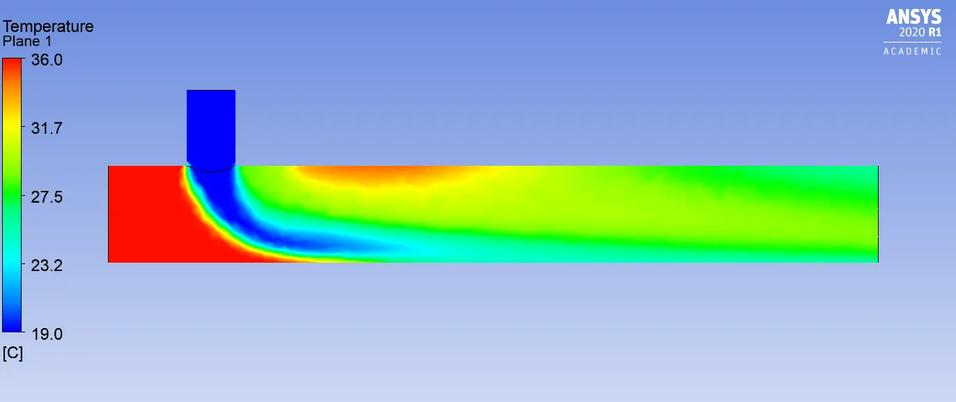
Momentum ratio=2 Hot inlet Temperature=36° Cold inlet Temperature=19° Hot inletair Velocity=3m/s Cold inlet air Velocity=12m/s (i.e Momentum ratio=4) RESULTS:- Residuals plot Area weighted average of temperature Standard deviation of temperature POST PROCESSING RESULTS:- Temperature contour along the pipe Temperature contour across the pipe Velocity contour along the pipe Velocity contour across the pipe Temperature line plot along the pipe Temperature line plot across the pipe Velocity line plot along the pipe Velocity line plot across the pipe

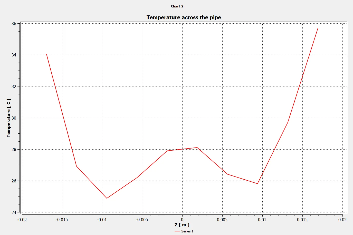
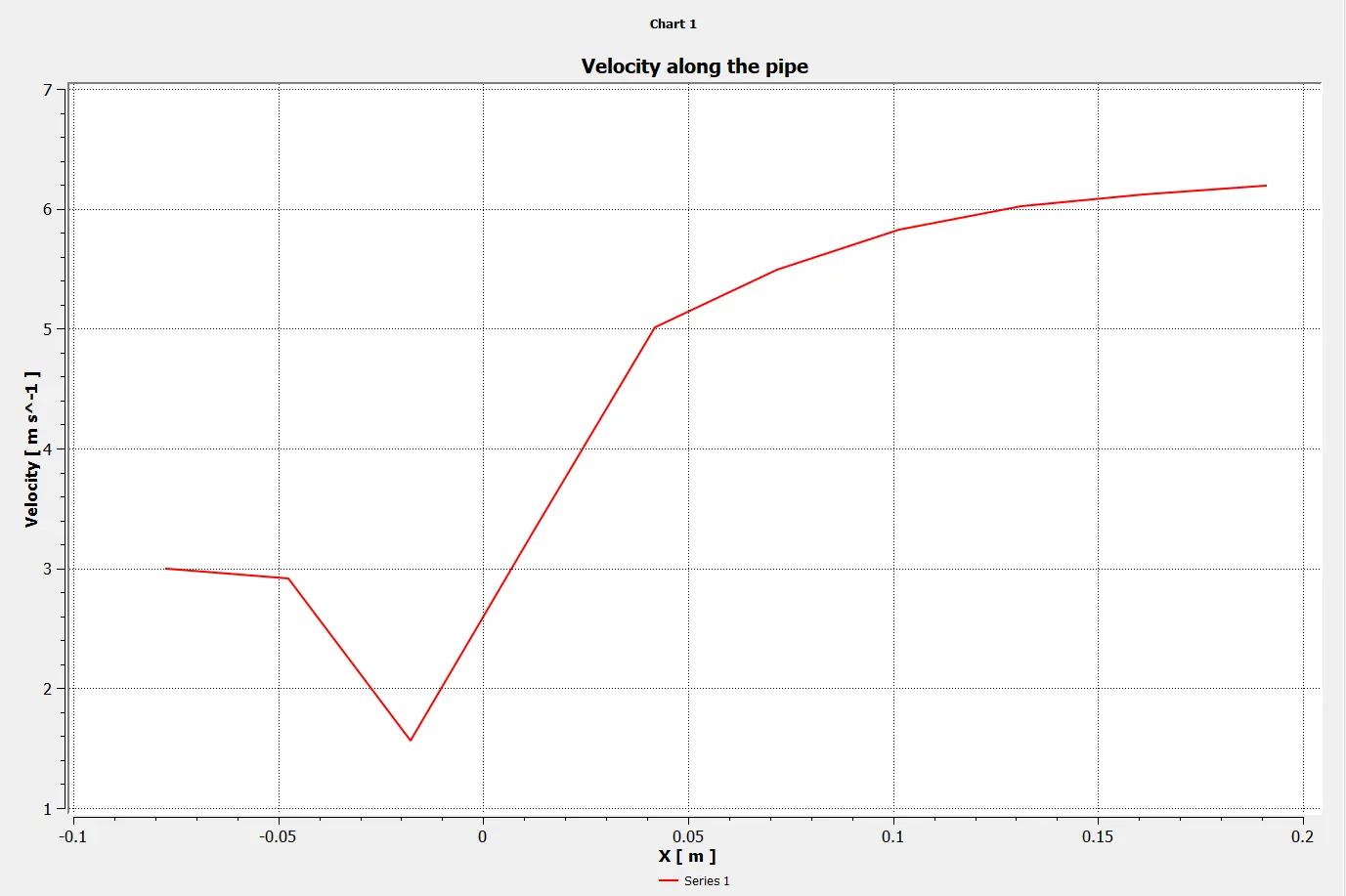
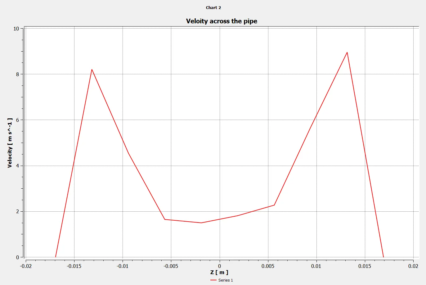
Comparision between K-Epsilon Short and Long tee

Geometry	Momentum ratio	Average outlet Temperature	Standard deviation
Short tee	2	30.48	1.5
Short tee	4	27.5	0.9
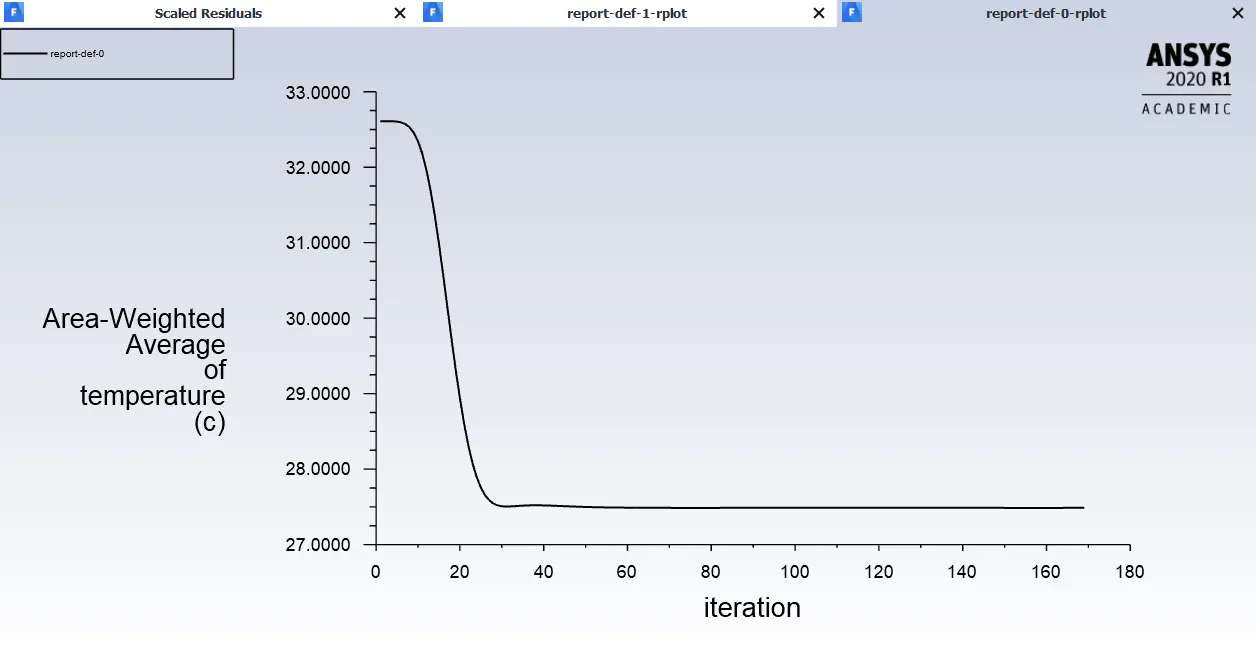
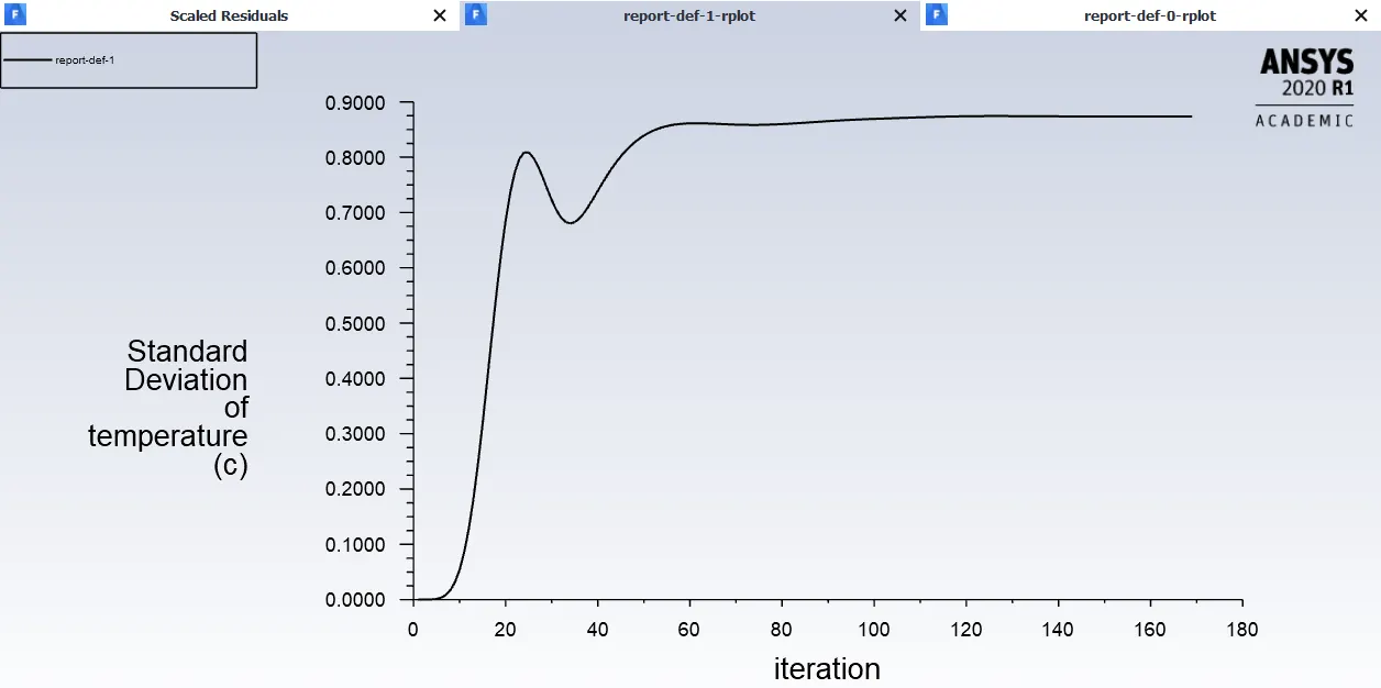
Long tee	2	30.40	1.5
Long tee	4	27.5	0.85

• From above table we can see that Average temperature and standard deviation are almost same for both short and long tee under K-Epsilon model.
• But for more efficiency short tee would be prefered.

MESH INDEPENDENT TEST:-

Geometry:-Short tee

In mesh independent test we put different element size for the shot mixing tee and compare the results.

Element size=5mm Mesh generation Residuals plot Area weighted average of temperature Standard deviation of temperature

Element size=10mm Mesh generation Residuals plot Area weighted average of temperature Standard deviation of temperature

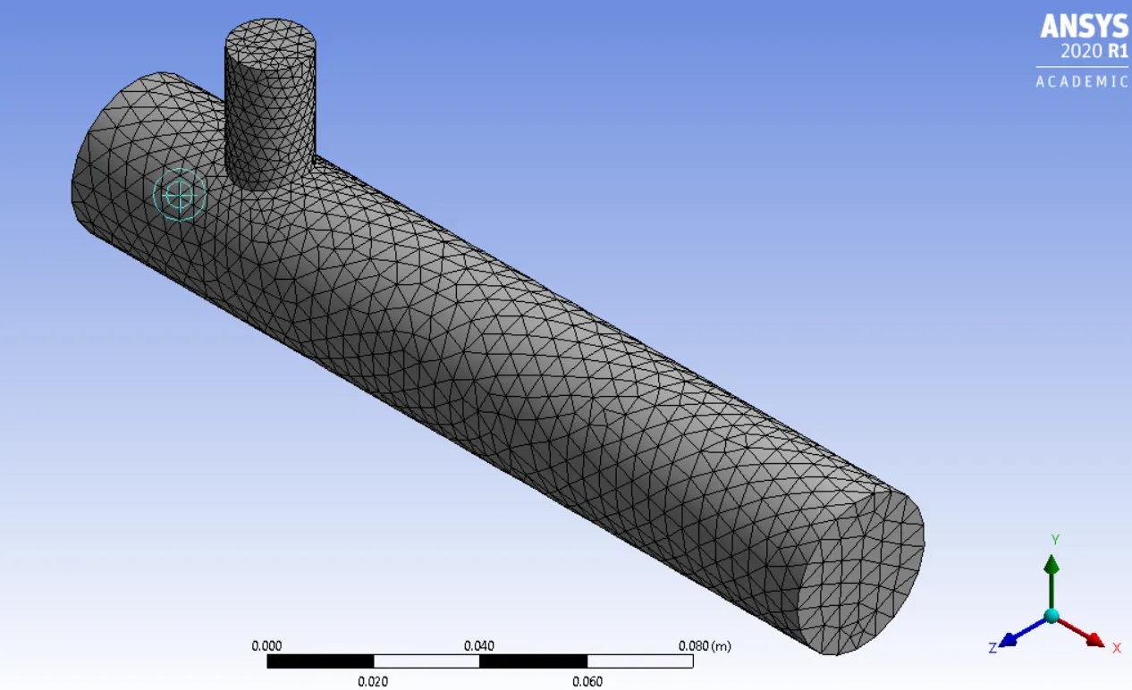
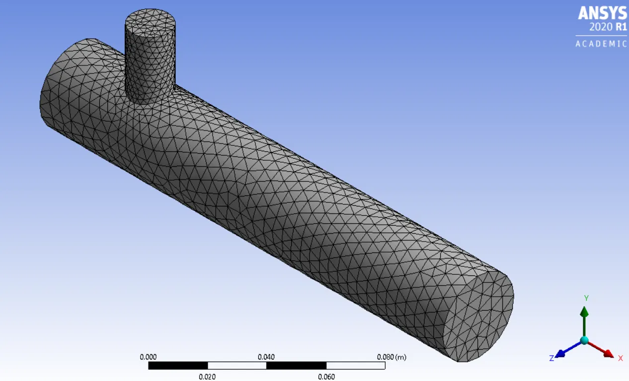
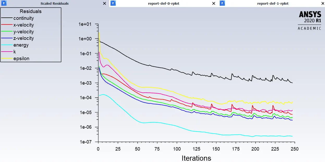
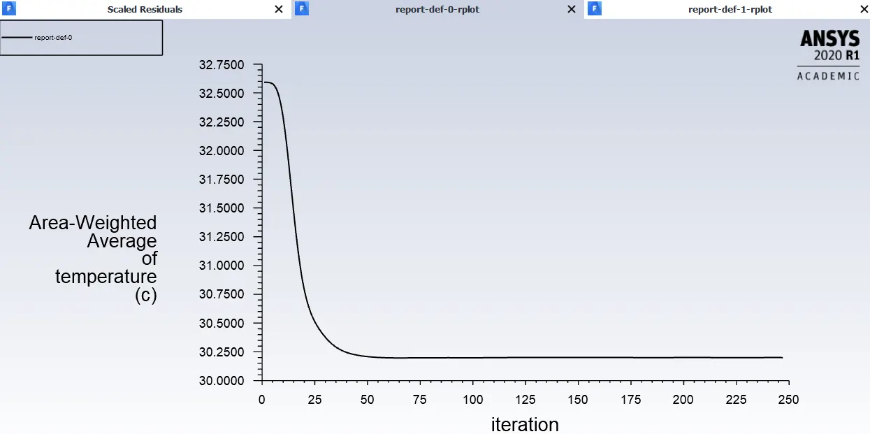
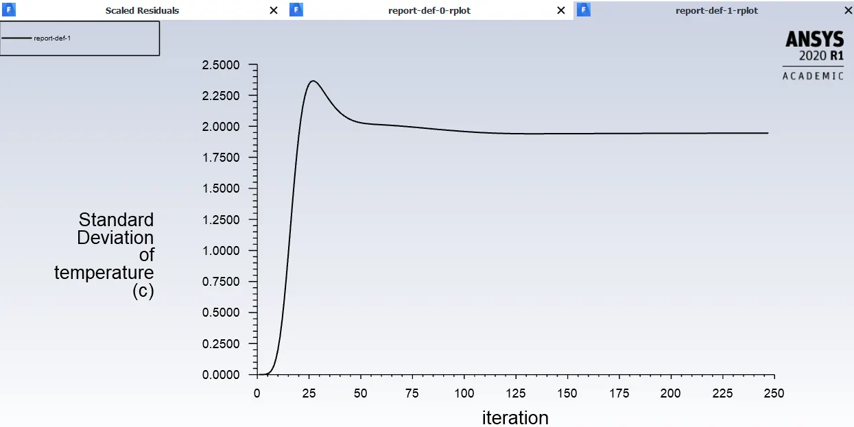
Comparission between different mesh size for short mixing tee

Mesh size	Number of elements	No of nodes	Iterations to converge	Average outlet temperature
2mm	105865	21347	220	30.5
5mm	14330	3152	More than 300 iterations	30.3
10mm	12760	2837	247	30.25

CONCLUSION:-

1) From the mesh independent test we can see that smaller the element size the accurate will be the results when compared to other bigger element size with analytical solutions.

• By decreasing the mesh size the average outlet temperature starts approaching towards analytical solution.
• Also residual errors decreases as we decrease the mesh size.

2) From the comparission between K-Epsilon short and long tee we can see that Maximum Efficiency of mixing tee does not depend on the length of the Mixing tee but depends on the velocity of cold inlet.

3) From Results we can tell that higher the Momentum ratio i.e,high cold inlet velocity can maximise the efficiency and best suitated for more applications.

• Increasing the Momentum ratio decreases the outlet temperature

===>>From above simulation results of Short and long tee under different turbulent models and Momentum ratio we can conclude that "To attain maximum Efficiency of Mixing tee, Short mixing tee with Momentum ratio 4 is best suited".