Steady Vs Unsteady flow over a cylinder
STEADY VS UNSTEADY FLOW OVER A CYLINDER
AIM:-
To Simulate the flow over a cylinder and explain the phenomenon of Karman vortex street.
OBJECTIVE:-
- To simulate the flow with the steady and unsteady case and calculate the Strouhal number for Reynolds number =100.
- To calculate the coefficient of drag and lift over a cylinder by setting the Reynolds number to 10, 100, 1000, 10000, 100000 under steady case.
- To discuss the effect of Reynolds number on the coefficient of drag.
THEORY:-
Phenomenon of Karman vortex street:
The Karman vortex street is an exquisite flow pattern that can be seen in a variety of flow situations, these are caused by a process known as vortex shedding, which is responsible for the unsteady seperation of fluid around blunt bodies.
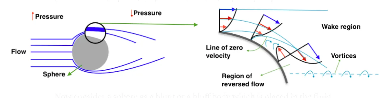
Now consider a sphere as a blunt which is placed in the fluid flow, we can see that there is boundary layer detachment i.e, flow seperation due to adverse pressure gradient. The decrease in the momentum of the flow is the primary cause of te adverse pressure gradient. Since the blunt body is symmetric in nature, the flow seperation is almost identical on the top half of the sphere and bottom half of the sphere. The pressure variations along the boundary layer are generated predominately due to the curved surface of the sphere. Vortices are also generated alongside recirculation in the region of eversed flow. These vortices start to swirl in a repeating manner. These low pressure alternating vortices tend to repeat at a certain frequency this is called frequency of vortex shedding.
PROCEDURE:-
Geometry:-
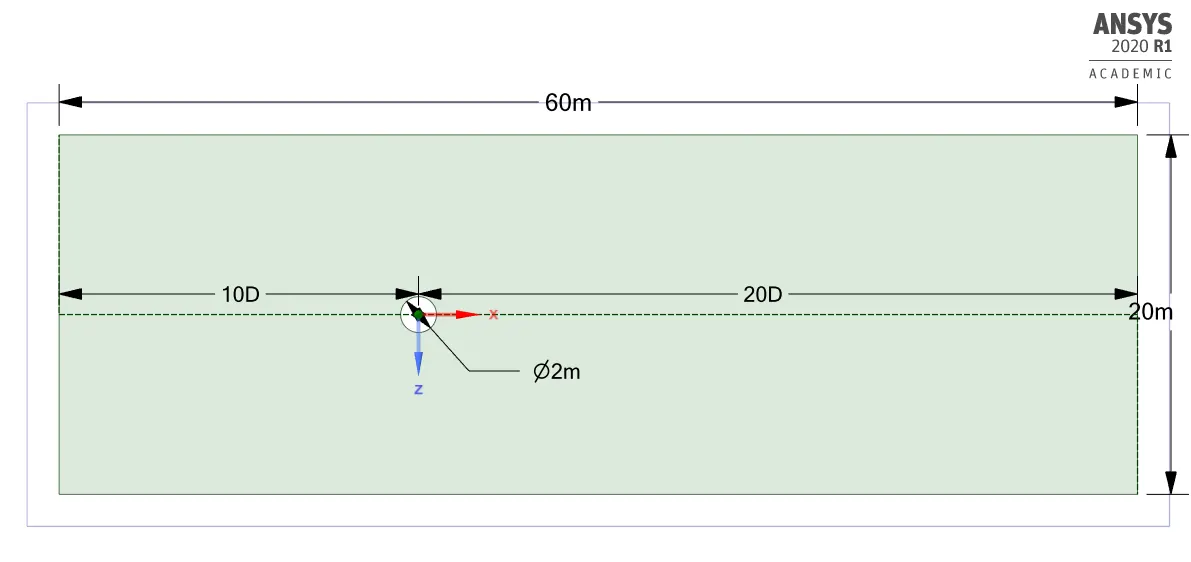
We have to dezign a 2D compuational domain in a Ansys spaceclaim as per given dimensions as shown in a below figure.
Meshing:-
- After the dezigning of 2D computational domain we need to mesh a model for further simulation.
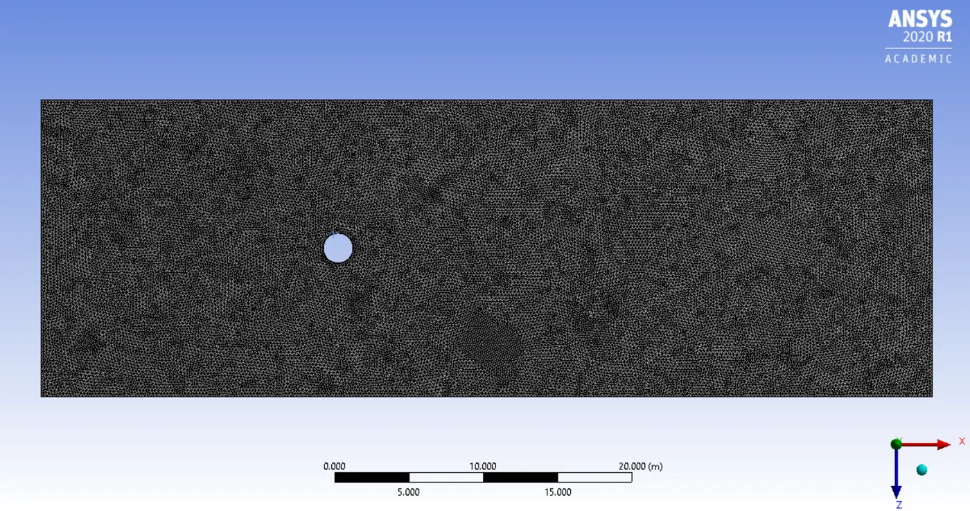
- By selecting generate mesh option in Ansys meshing it Meshs the whole model but, it normaly creates quadilateral dominant mesh, we need to convert it into a triangle dominant mesh. This can be done by inserting a method. Select a method option and select the face where we want to mesh and select triangle type of mesh with element size of 0.2m.
| Element size | 0.2m |
| Number of nodes | 31883 |
| Number of elements | 62714 |
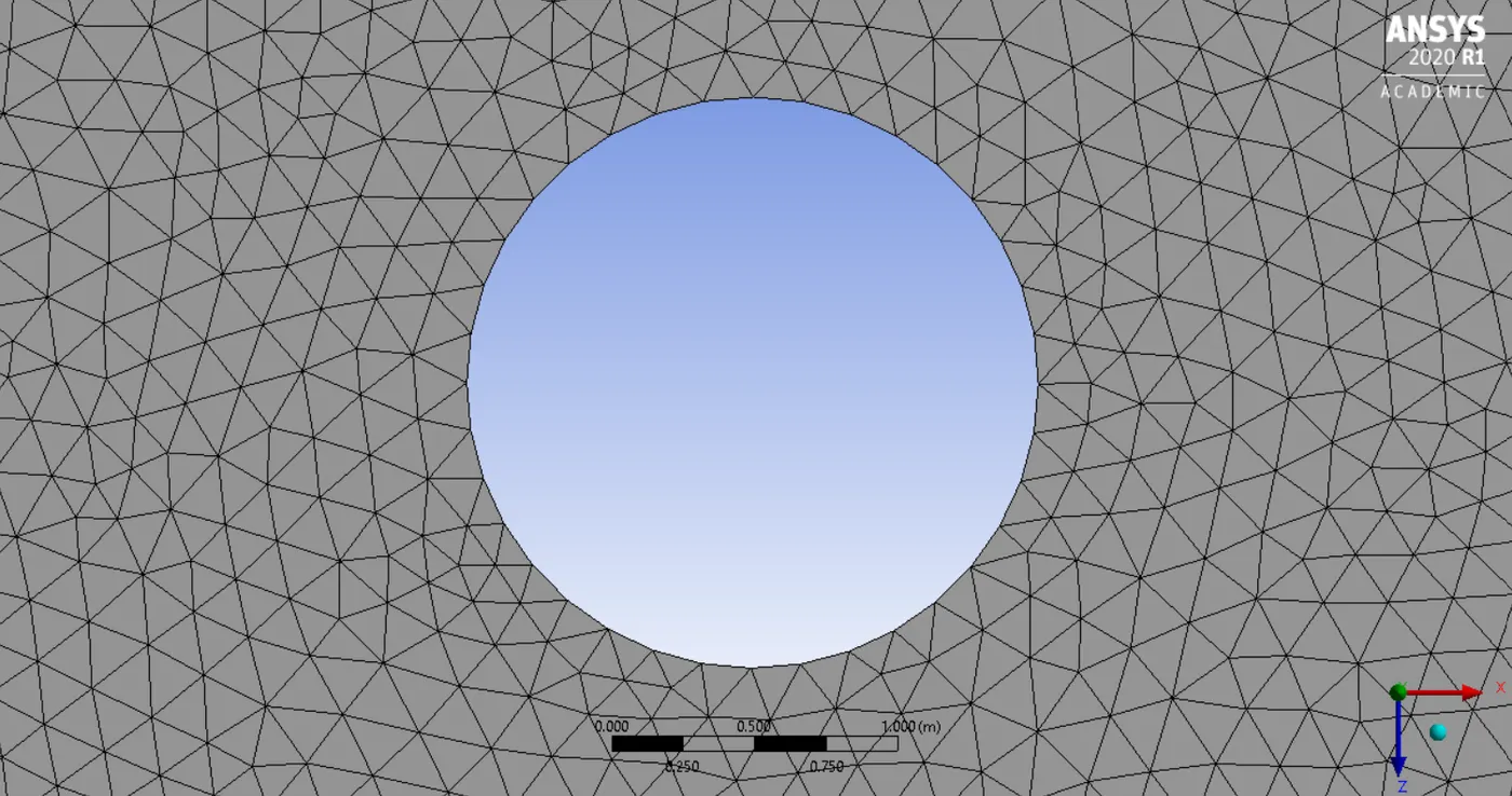
- The cylinder we have is not perfectly circular if we proceed with this kind of mesh then we might get wrong outputs so we need to divide the circle into many number of division which gives us the smooth curve as shown in below figure. This can be done by edge sizing options then we need to select the number of division type, and we have to put how many division we require to get smooth curve. here, we give number of dividions= 36.
- To resolve boundary over a cyclinder we require finner mesh around the cyclinder. This can be done by inserting inflation in boundary scooping method we need to select the edge of the circle and select first layer thickness in inflation option.
| First layer height | 0.005m |
| Maximum layer | 6 |
| Growth rate | 1.2 |
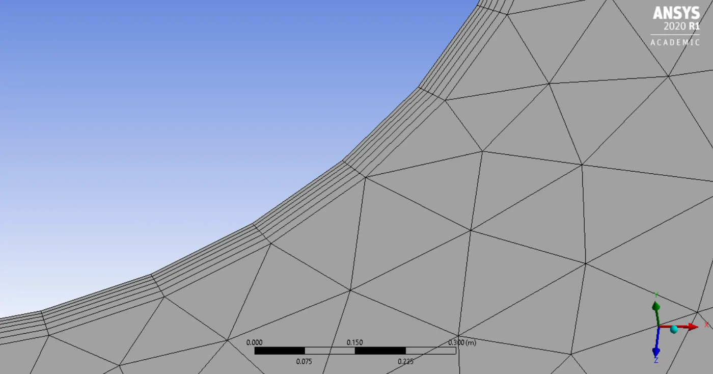
PART 1===>> To simulate the flow with the steady and unsteady case and calculate the strouhal No. for Re=100
Case setup:-
- Here,we need to setup a solver.
- The solver type is pressure based and velocity formation is absolute and based on the case study we have to select the steady state or transient state condition.
- After the solver setup, in physics we need to select laminar viscous model.
- Then we need to create a user defined material whose
- density= 1kg/m^3
- Viscosity= 0.02kg/m-s
- Velocity= 1m/s (Re No.=100)
Boundary conditions:-
- After selecting viscous model and solver setup we need to assaign boundary conditions to the different parts of cylinder. Since, we have already assaigned the name for the boundaries it automatically selects the boundary conditions. Then in edit option we can feed the inlet velocity.
- Then we need to create a monitor point so that we can see the vertex average of velocity magnitude at that point.
- Then we need to plot a drag and lift coefficient graph by selecting definitions option.
- Then we need to plot velocity and pressure contour plot by selecting it in contour option.
- For Steady state----> Hybrid initialization
- For Transient state--->Standard initialization and Time step size is 0.1s.
RESULTS:-
|
STEADY STATE Residuals plot
Vertex average Drag coefficient Lift coefficient Velocity contour plot Pressure contour plot |
TRANSIENT STATE Residuals plot
Vertex average Drag coeficient Lift coefficient Velocity contour plot Pressure contour plot |
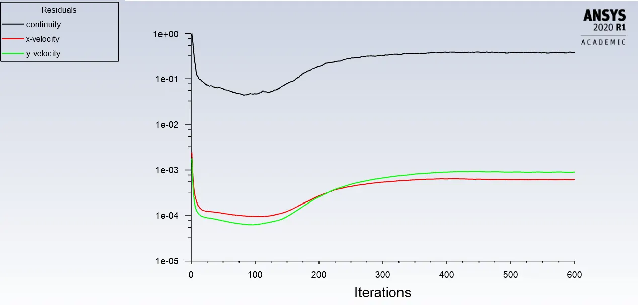
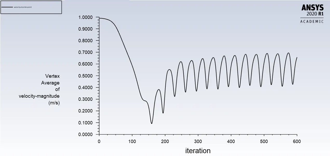
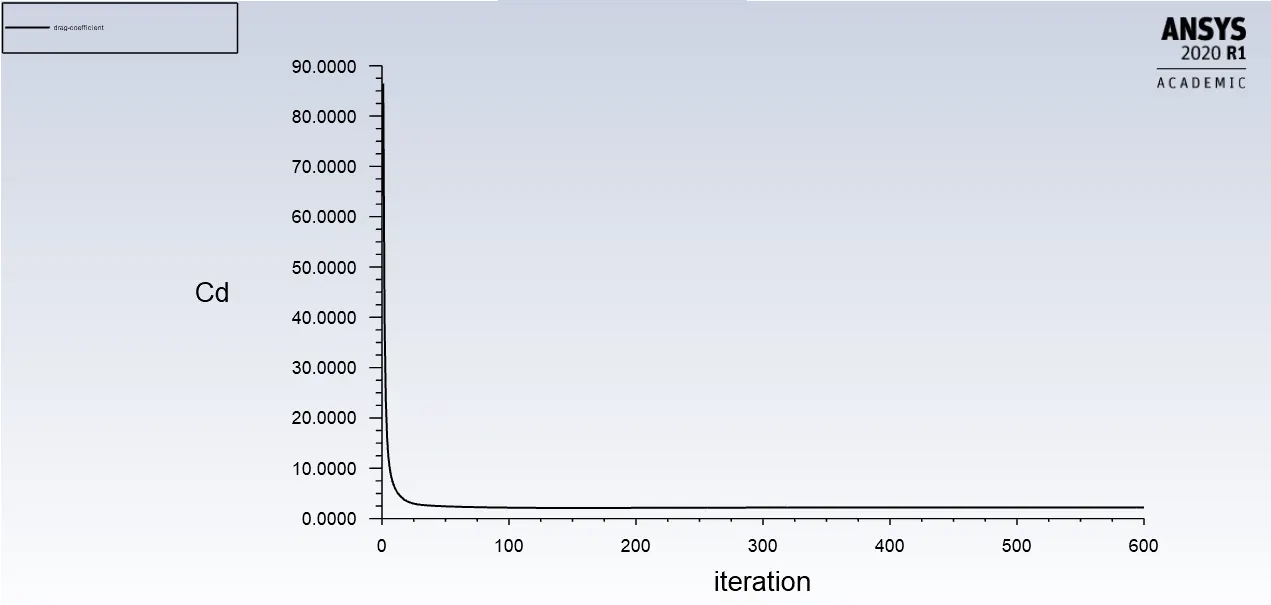
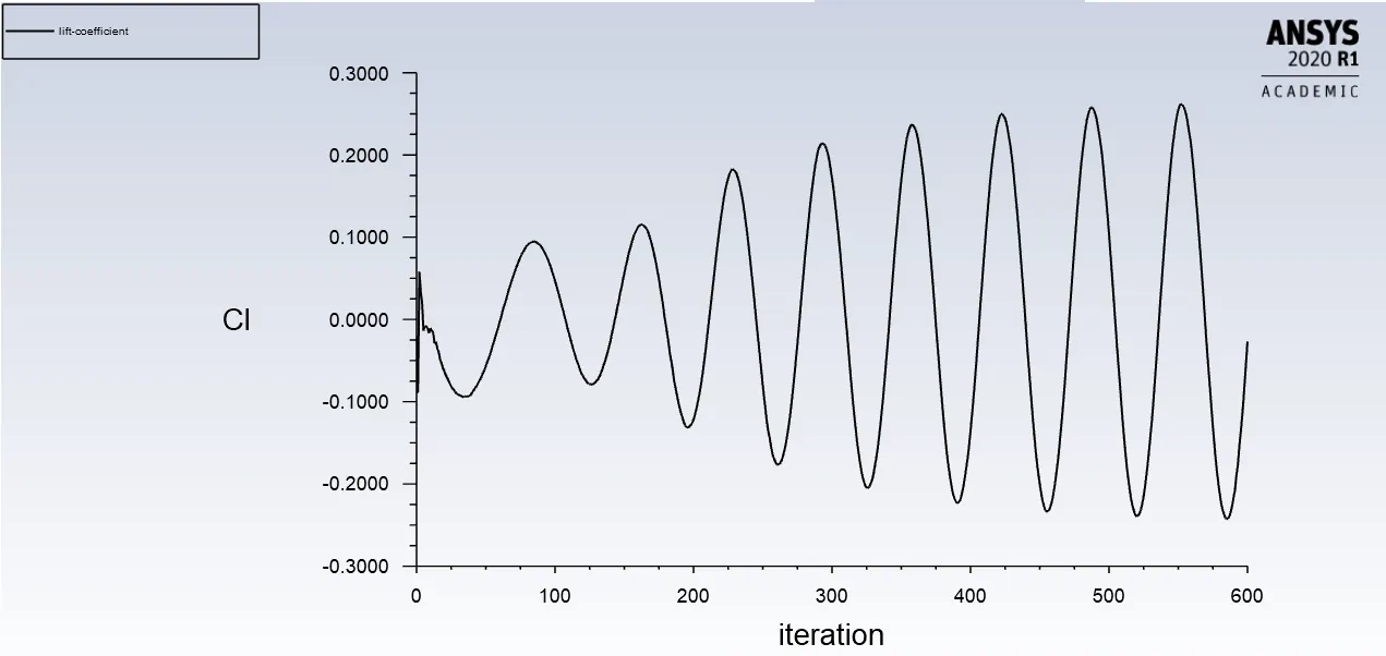
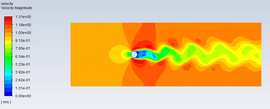
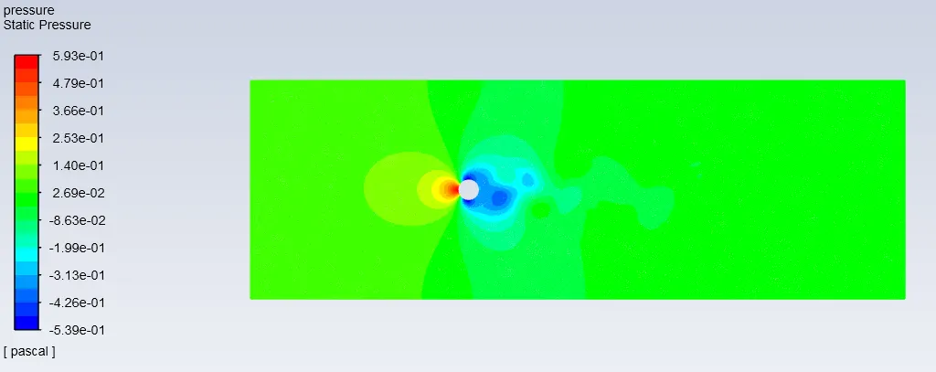
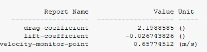
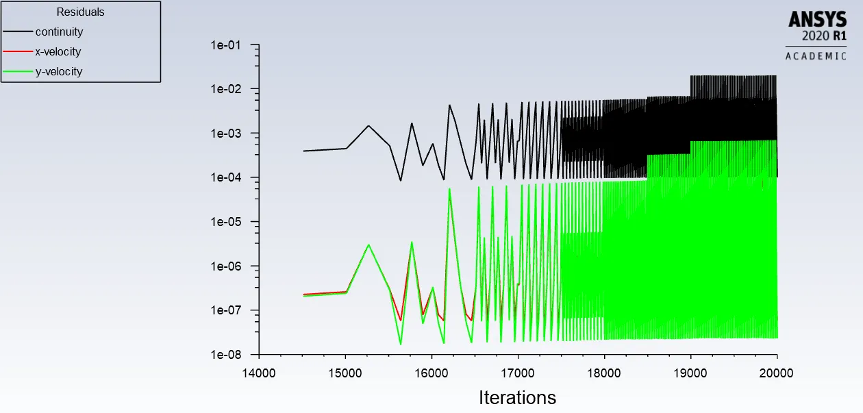
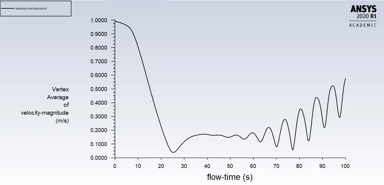
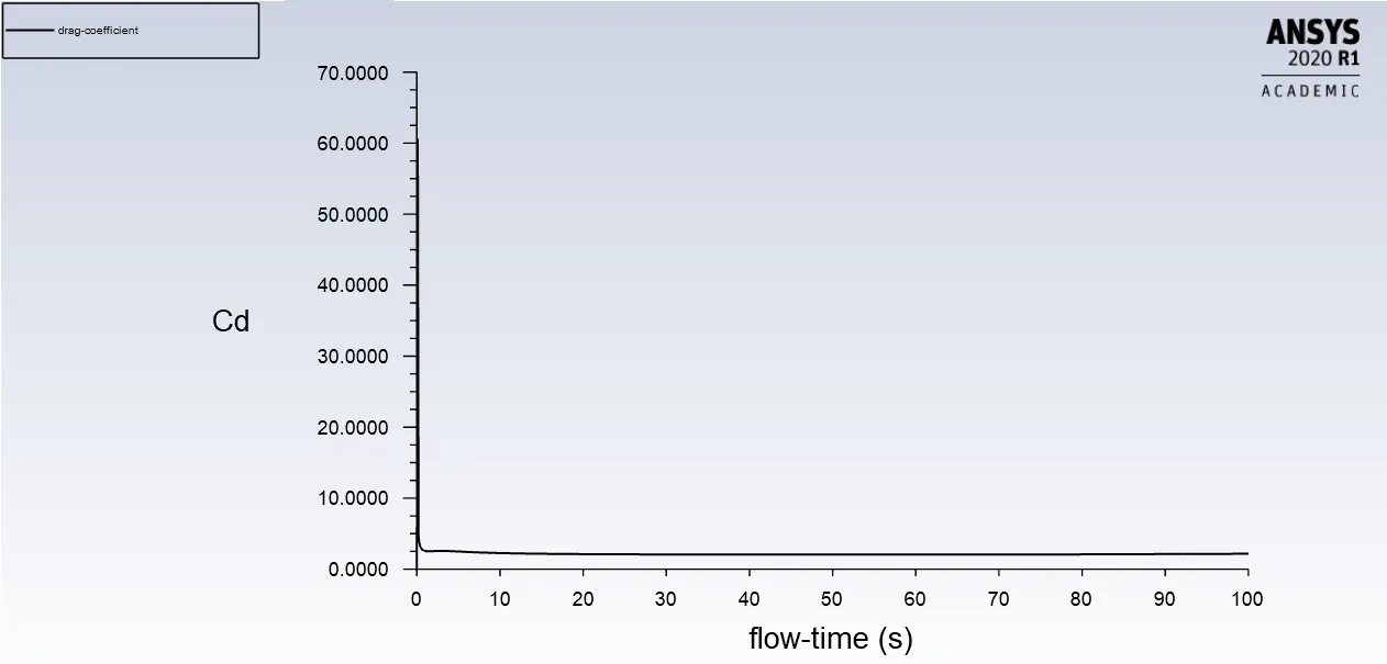
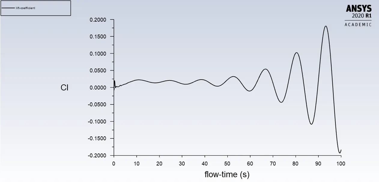
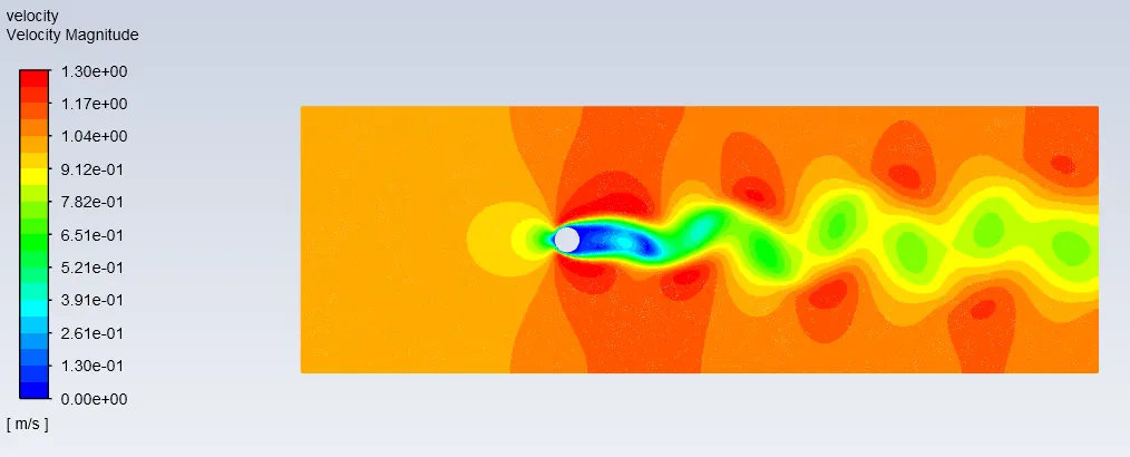
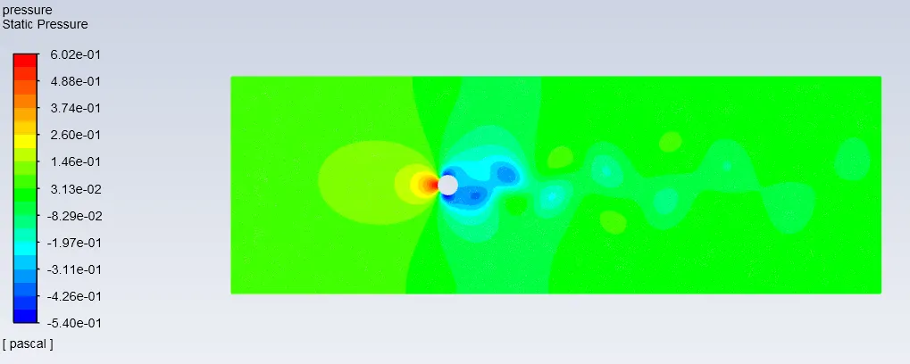
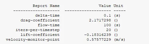
| Case | Vertex Average | Drag coefficient | Lift coefficient |
| Steady state | 0.6577m/s | 2.1988 | -0.02674 |
| Transient state | 0.5757m/s | 2.1717 | -0.18316 |
Strouhal number
- In dimensional analysis Strouhal number is a dimensionless number describing oscilating flow mechanisms. Strouhal number represents the ratio of inertial forces due to local acceleration of the flow to the inertial forces due to the convective acceleration.
- In periodic motion Strouhal number is asociated with the oscillations of the flow due to inertial forces relative to the changes in velocity due to the cnvective acceleration of the flow field.
- Strouhal number is better suited to periodic flows the expression for that is given below.
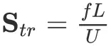
- Where, f is the frequency of the oscillations(vortex shedding)
- L is characteristics length, in our case we take diameter of circle.
- U is the velocity of fluid.
For Steady state:-
We cannot find the frequency as there is no time parmeter involved.
For Transient state:-
- L=2m
- U=1m/s
- f= we manually calculate the no of frequency by number of maximum amplitude(peaks) of the cycle divided by total duration of time taken to complete this cycle.
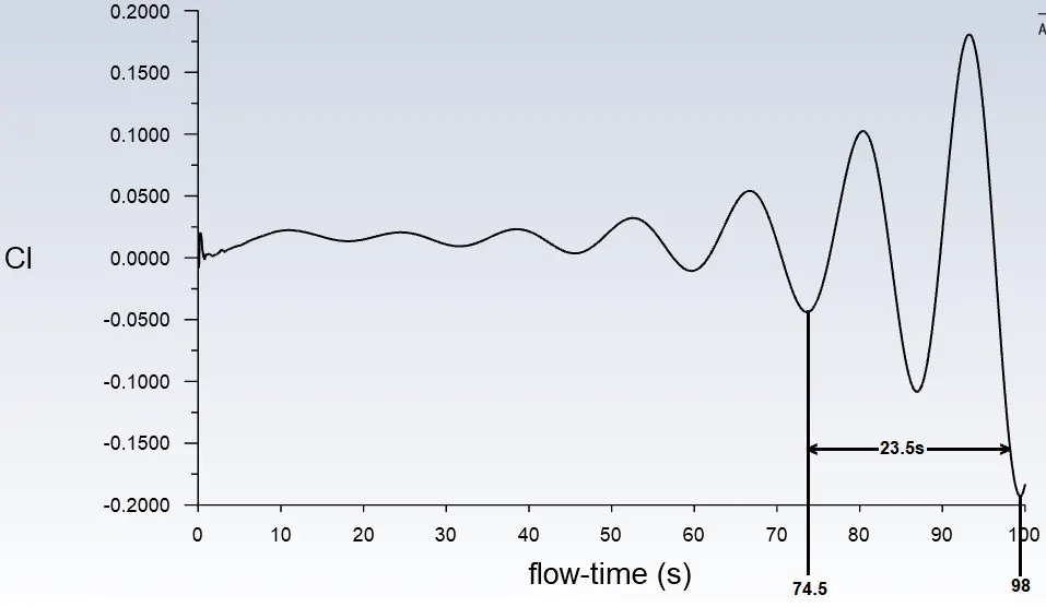
f = 2/23.5 =0.0851Hz
St =(0.0851 * 2)/1 = 0.1702
PART 2===>> To calculate the coefficient of drag and lift over a cyclinder by setting the Reynolds number to 10, 100, 1000, 10000, 100000 and to run with Steady state, and to discuss the effect of Reynolds number on the coefficient of drag.
Drag coefficient- The drag coefficient is a dimensionless quantity that is used to quantify the drag or resistance of an object in a fluid environment,such as air or water. The drag coefficient is always associated with a particular surface area. The drag coefficient of any object comprises the effect of the two basic contributors to fluid dynamic drag, skin friction and form drag.
The drag coefficient is defined as
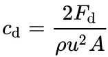
where, Fd is the drag force, rho is the mass density, u is the flow speed, A is the reference area.
Lift coefficient- The lift coefficient is a dimensionless coefficient that relates the lift generated by a lifting body to the fluid density around the body, the fluid velocity and an associated reference area. The lift coefficient contins the complex dependencies of object shape on lift.
Te lift coefficient is defined as
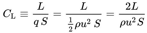
Where, L is the lift force, S is the surface area, rho is the fluid density and u is flow speed.
Geometry, Mesh, Case setup:-
- All are same as in the above case i.e, Part 1
- But while, selecting viscous model for Reynolds number(10, 100, 1000)use laminar viscous model and for Reynolds number(10000, 100000)use K-omega viscous model, because as the reynolds no increases above 2000 it becomes turbulet so it is better to use K=omega viscous model.
Reynolds number =10
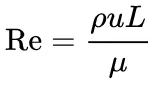
- Viscosity=0.2kg/m-s
- Velocity=1m/s
- Density= 1kg/m^3
- L=2m (diameter)
|
Residuals plot:- |
|
Vertex average of velocity magnitude plot:- |
|
Plot of Drag coefficient:- |
|
Plot of Lift coefficient:- |
|
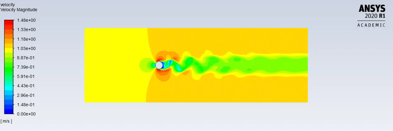
Velocity contour plot:- |
|
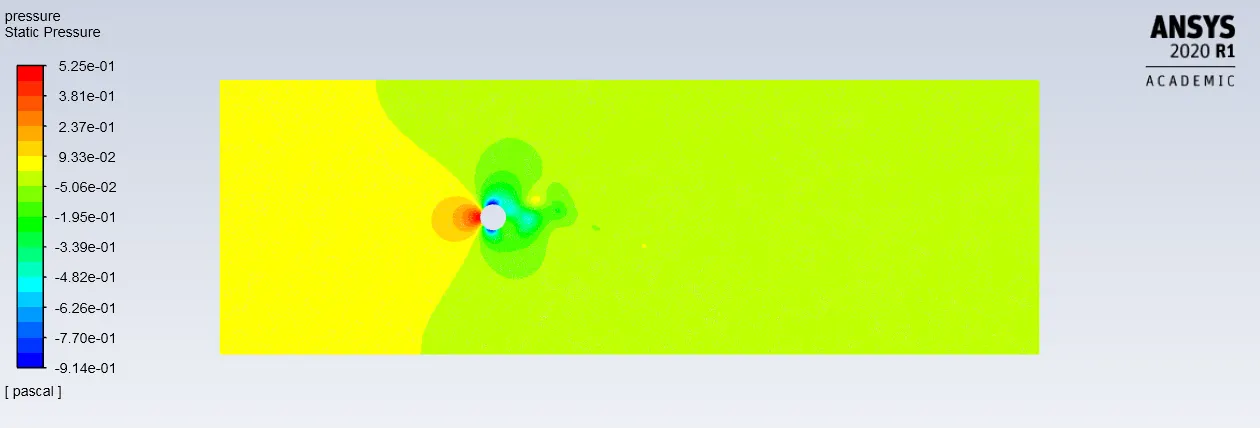
Pressure contour plot:- |
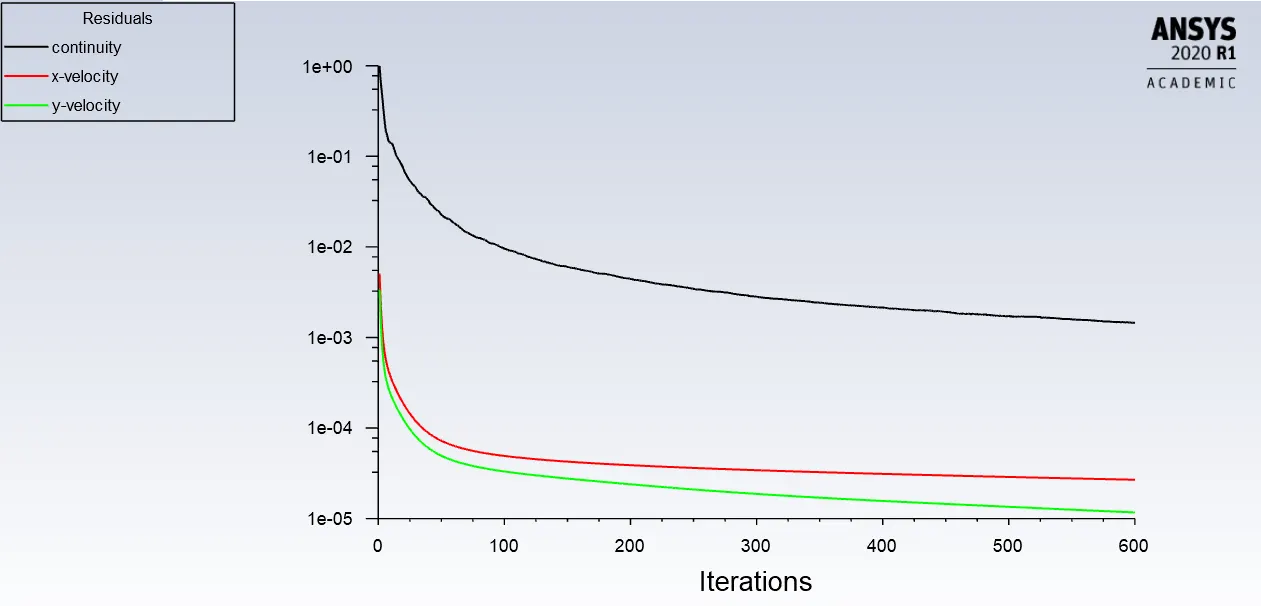
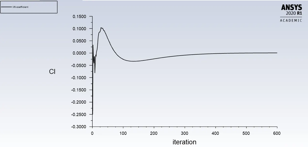
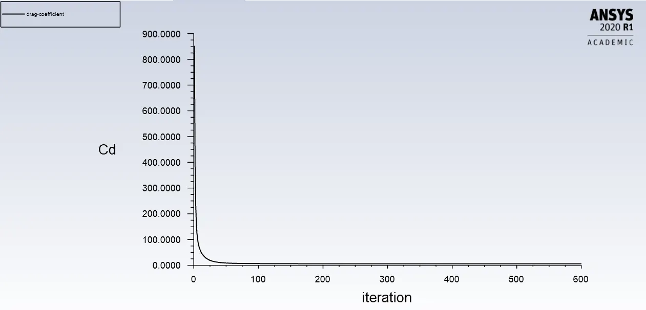
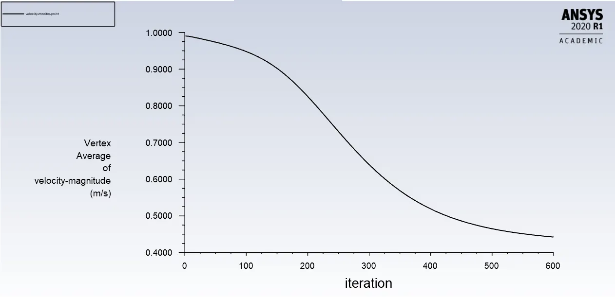
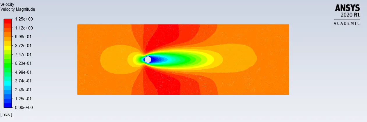
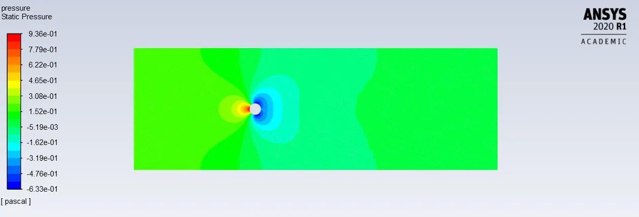
Reynolds number =100
- Viscosity=0.02kg/m-s
- Velocity=1m/s
- Density= 1kg/m^3
- L=2m (diameter)
|
Residuals plot:- |
|
Vertex average of velocity magnitude plot:- |
|
Plot of Drag coefficient:- |
|
Plot of Lift coefficient:- |
|
Velocity contour plot:- |
|
Pressure contour plot:- |
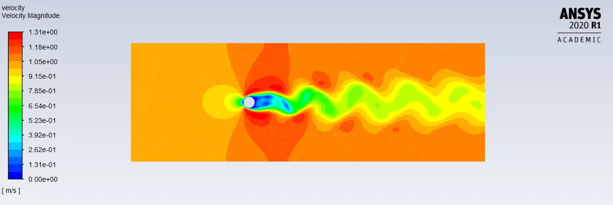
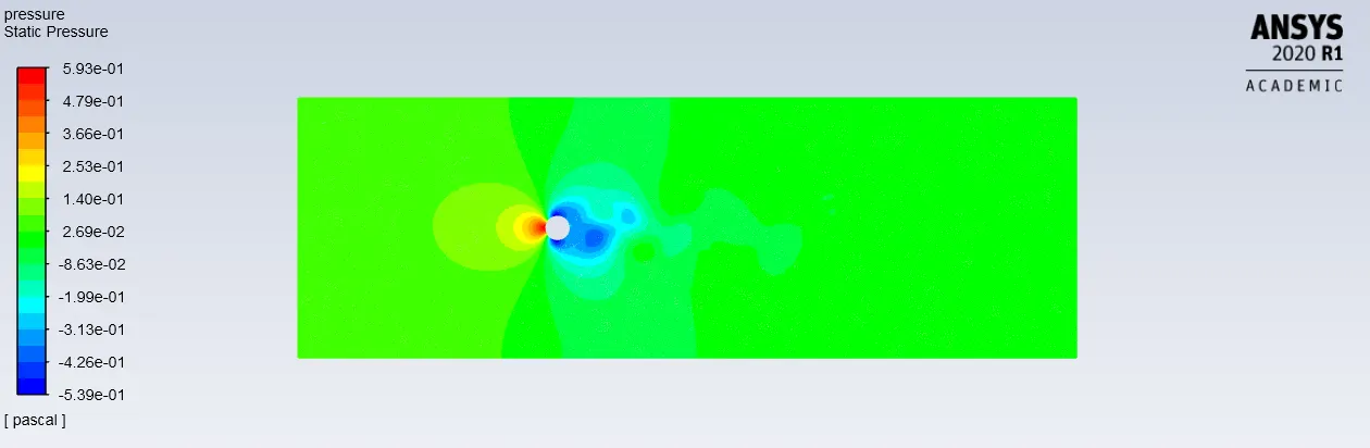
Reynolds number =1000
- Viscosity=0.002kg/m-s
- Velocity=1m/s
- Density= 1kg/m^3
- L=2m (diameter)
|
Residuals plot:- |
|
Vertex average of velocity magnitude plot:- |
|
Plot of Drag coefficient:- |
|
Plot of Lift coefficient:- |
|
Velocity contour plot:- |
|
Pressure contour plot:- |
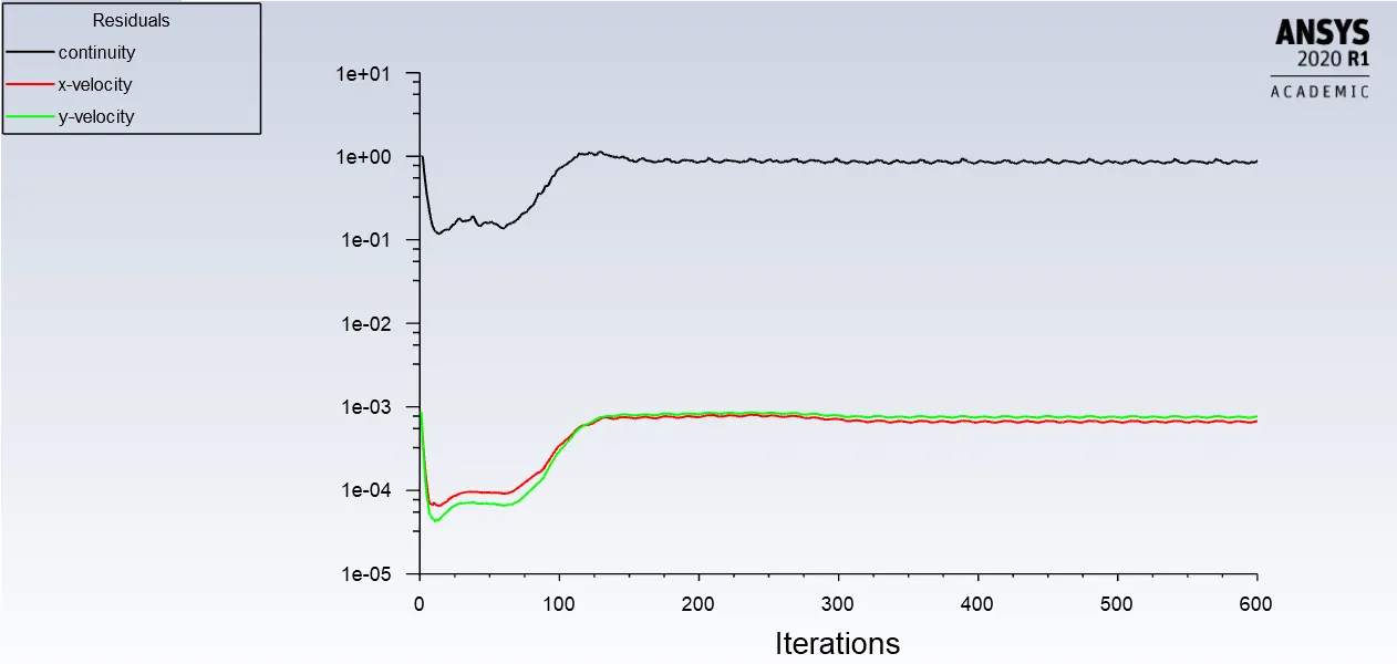
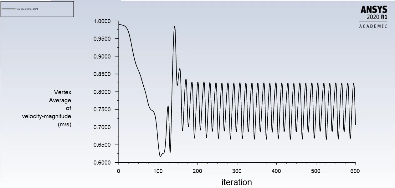
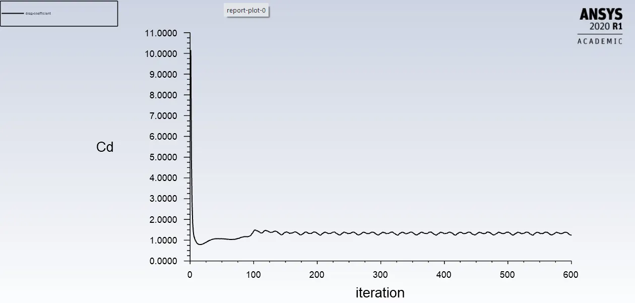
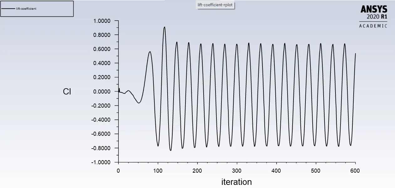
Reynolds number =10000
- Viscosity=0.0002kg/m-s
- Velocity=1m/s
- Density= 1kg/m^3
- L=2m (diameter)
|
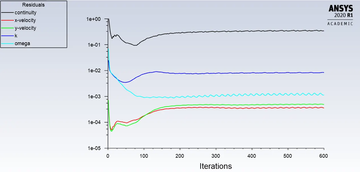
Residuals plot:- |
|
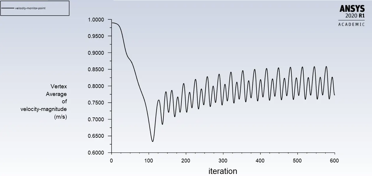
Vertex average of velocity magnitude plot:- |
|
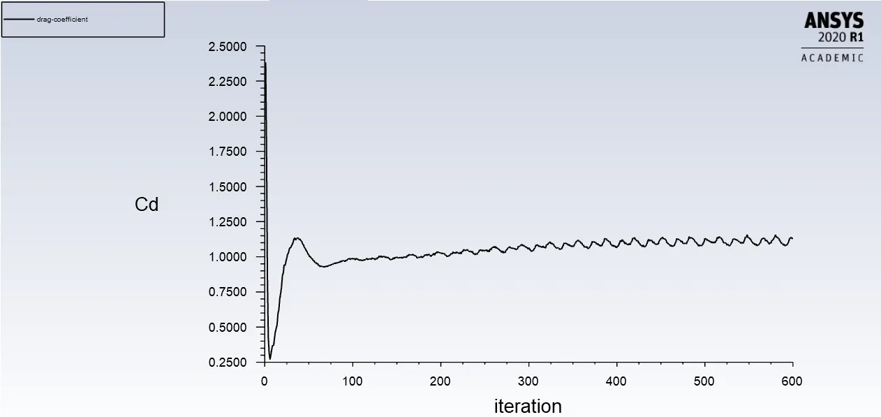
Plot of Drag coefficient:- |
|
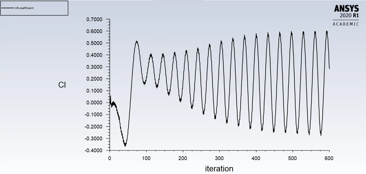
Plot of Lift coefficient:- |
|
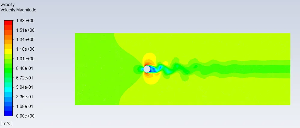
Velocity contour plot:- |
|
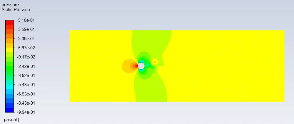
Pressure contour plot:- |
Reynolds number =100000
- Viscosity=0.00002kg/m-s
- Velocity=1m/s
- Density= 1kg/m^3
- L=2m (diameter)
|
Residuals plot:- |
|
Vertex average of velocity magnitude plot:- |
|
Plot of Drag coefficient:- |
|
Plot of Lift coefficient:- |
|
Velocity contour plot:- |
|
Pressure contour plot:- |
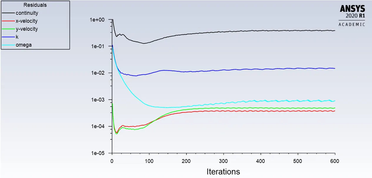
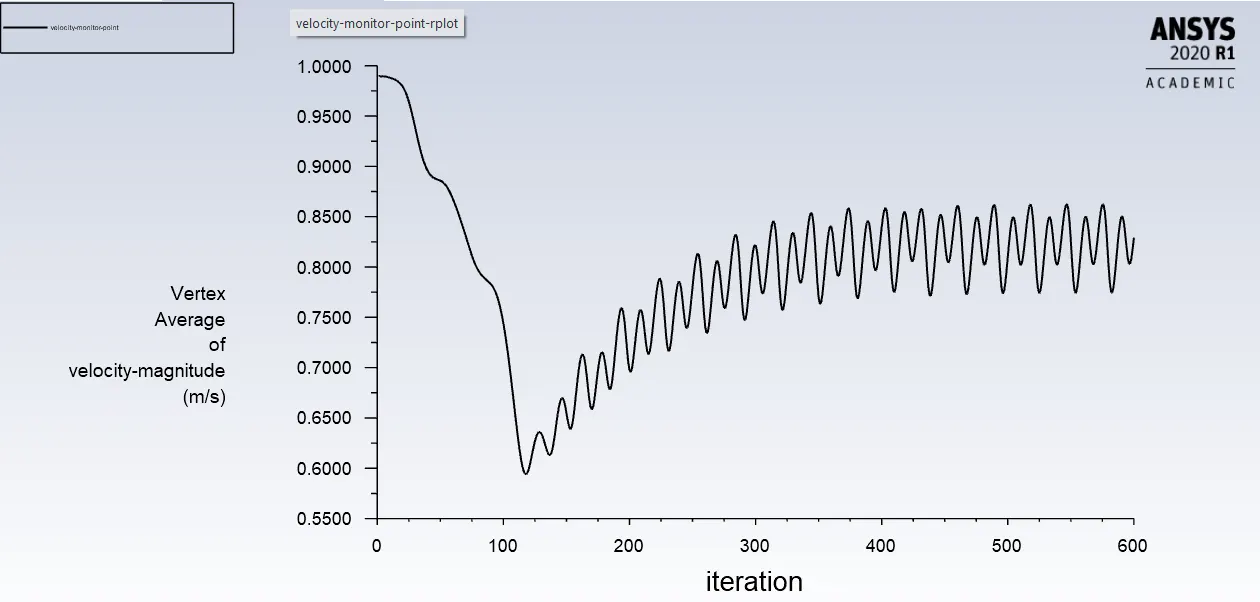
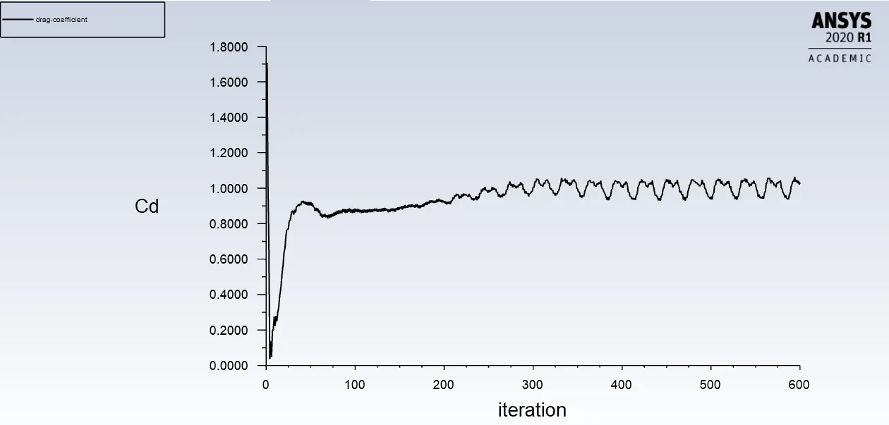
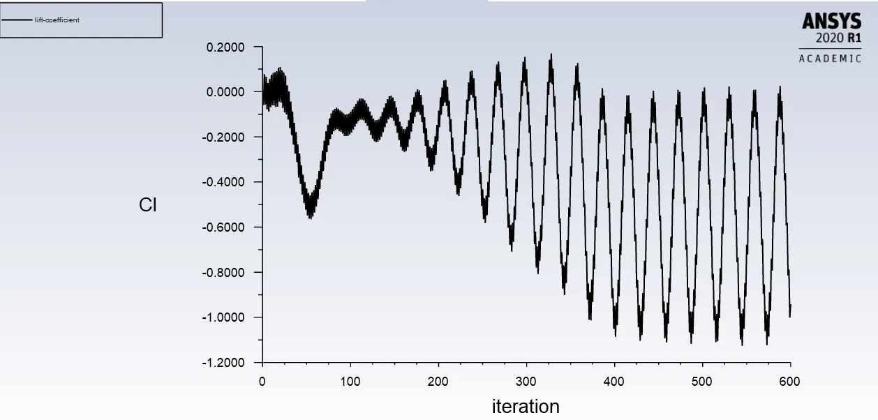
| Reynolds number | Drag coefficient | Lift coefficient | Vertex average |
| 10 | 5.4529 | 0.0006091 | 0.44241 |
| 100 | 2.1988 | -0.026743 | 0.6577 |
| 1000 | 1.2610 | 0.53856 | 0.7058 |
| 10000 | 1.1285 | 0.28348 | 0.7734 |
| 100000 | 1.0325 | -0.94179 | 0.8291 |
CONCLUSION:-
Part 1:-
- From above Residuals plot we can see that flow is converging for both steady and transient state. But to calculate strouhal number transient state is better because it gives solution at every time step.
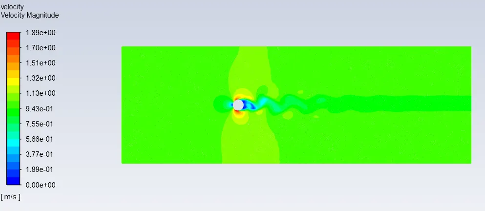
- From above velocity contour plot we can clearly observe the phenomenon of Karman vortex street.
- From the results strouhal number is calculated as 0.1702
Part 2:-
- Different simulations has been run successfully to observe the behaviour of drag coefficient with respect to Reynolds number.
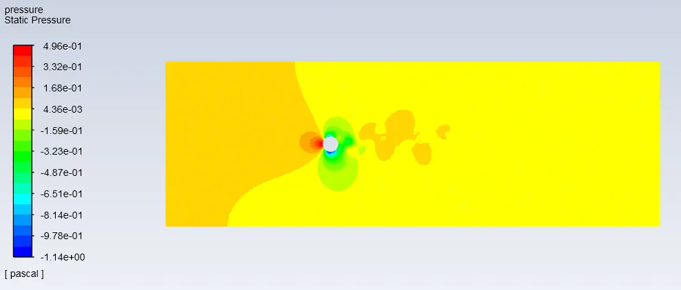
- From above results we can observe that vertex shedding happens in all the cases except in the Reynolds number of 10 and also we can see that as the reynolds number increases the vertex average also increases at a monitor point.
- From above results we can clearly see the variation in the drag as the Reynolds number increases Drag coefficient decreases.