Exhaust Port Challenge

AIM:-

To understand the conjugate heat transfer and to perform CHT analysis on an exhaust port.

OBJECTIVES:-

• To give a brief description of why and where a CHT analysis is used.
• To maintain the y+ value according to the turbulence model and to justify the results.
• To calculate the wall/surface heat transfer coefficient on the internal solid surface & show the velocity & temperature contours in appropriate areas.
• To verify if the HTC predictions from the simulations are right and on what factors does the accuracy of the prediction depend on?

INTRODUCTION:-

• The Conjugate Heat Transfer (CHT) analysis type allows for the simulation of heat transfer between solid and fluid domains by exchanging thermal energy at the interfaces between them. The exchange of thermal energy between the two physical bodies is called the study of heat transfer.
• In solids, conduction often dominates whereas in fluids, convection usually dominates. Conjugate heat transfer is observed in many situations. For example, heat sinks are optimized to combine heat transfer by conduction in the heat sink with the convection in the surrounding fluid.

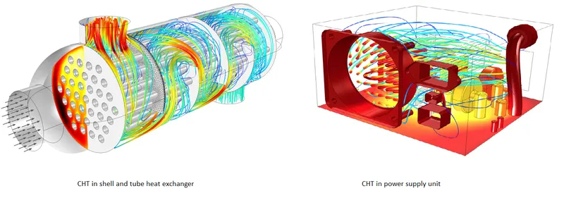
Modes of heat transfer

Conduction: diffusion of heat due to temperature gradients. A measure of the amount of conduction for a given gradient is the heat conductivity.

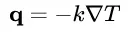
Convection: when heat is carried away by moving fluid. The flow can either be caused by external influences, forced convection; or by buoyancy forces, natural convection. Convective heat transfer is tightly coupled to the fluid flow solution.

Radiation: transfer of energy by electromagnetic waves between surfaces with different temperatures, separated by a medium that is at least partially transparent to the (infrared) radiation. Radiation is especially important at high temperatures, e.g. during combustion processes, but can also have a measurable effect at room temperatures.

Apllications of conjugate heat transfer

Heat exchanger:- A heat exchanger is a system used to transfer heat between two or more fluids. The fluids may be separated by a solid wall to prevent mixing. Forced convection is the most common way to achive a high heat transfer coefficient.

Heat sink:-A heat sink is a passive heat exchanger that transfers the heat generated by an electronic or a mechanical device to a fluid medium, often air or a liquid coolant through convection.

Solving and modeling approach

Modelling approach is divide into two cases baseline mesh and refined mesh

Geometry:-

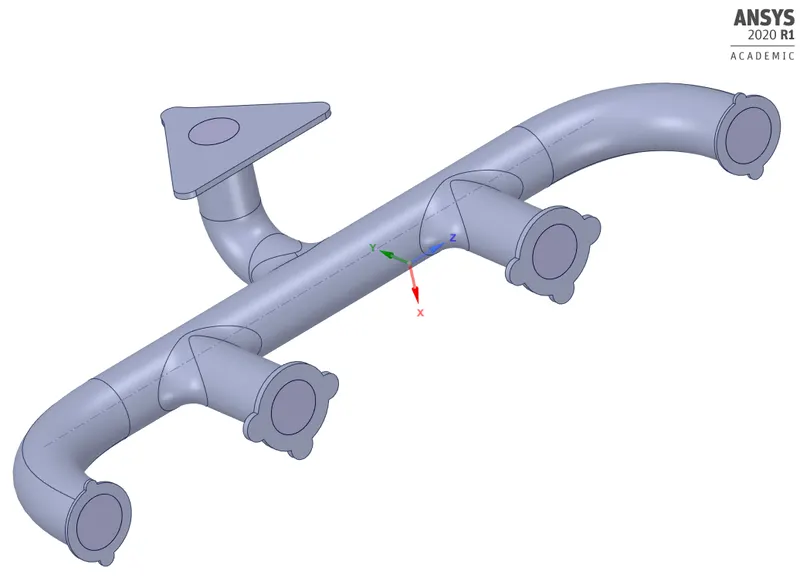
• The below figure 1 is the actual solid part of the component. Then we need to extract fluid domain from it.

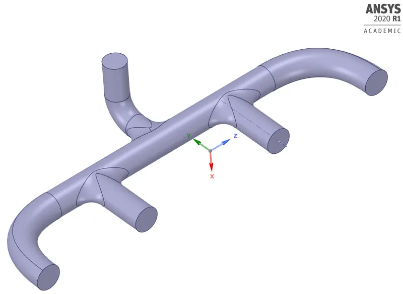
• The below figure 2 is the extracted fluid domain of the component.

CASE 1:- Baseline mesh

Meshing:-

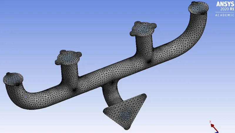
Here we need to name the boundaries using named selection option as inlet, outlet and outer wall convection. Then we need to generate mesh. Here we use baseline mesh to check the setup.

Element size	150mm
Number of nodes	28119
Number of elements	141472

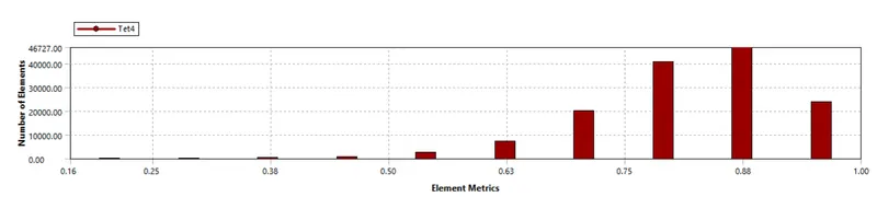
Mesh quality:-

Setup:-

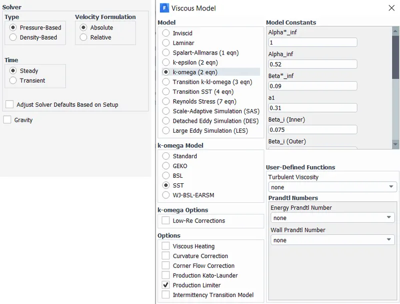
• Here we need to setup a solver. The solver type is pressure based steady state and absolute velocity formation.
• After the solver setup we need to select K-Omega SST turbulence model. K-omega sst model uses K-epsilon model in freestream section of fluid flow and uses K-omega model for the near wall computations. K-omega SST model is good for attaining thermal behaviour near the inner wall.

Boundary conditions:-

• After selecting the viscous model we need to assaign the boundary conditions to different part of component. Since we have already named the parts it automatically selects the boundary conditions.
• for inlet it is velocity inlet with velocity magnitude of 5m/sec and temperature of air is 700K
• for outlet it is pressure outlet with pressure gauge of 0pa.
• for outer wall convection it is thermal convection with heat transfer coefficient of 20 WK/m^2.
• Then we need to initialize the solver with hybrid initialization method and setup the number of iterations.

RESULTS:-

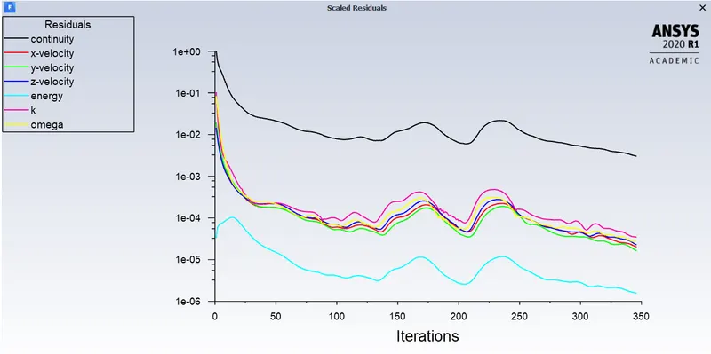
Residuals plot:-

Post processing results:-

Temperature contour at outer wall:-

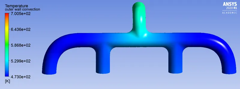
Velocity streamline:-

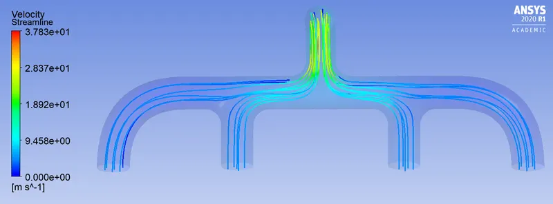
Temperature contour:-

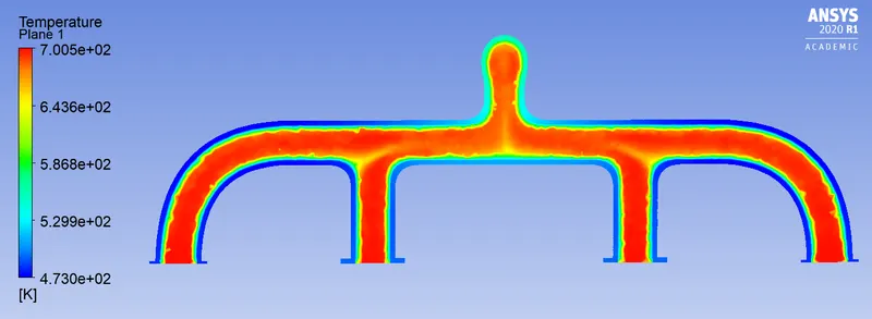
Heat transfer coefficient at outer wall:-

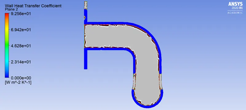
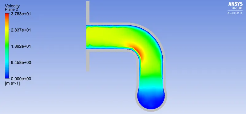
Velocity contour:-

CASE 2:- Refined mesh

Meshing:-

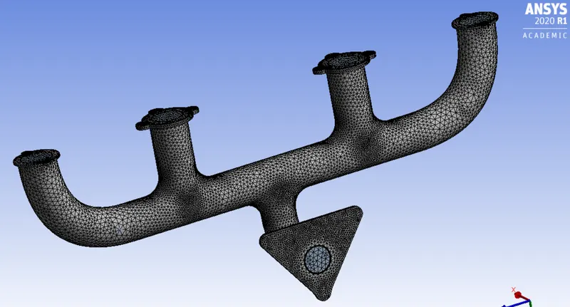
• For refinment of mesh we add inflation layers to get accurate reults near the wall and also we add body sizing for refinement.
• Thickness of inflation layer depends on the turbulence model. When we take K-Omega SSt model y+ ranges between 1-5 and sometimes below 1.
• We can find first layer thickness value using y+ value for a given density velocity and viscosity.

• Element size 150mm (Fluid domain)
• Body sizing 10mm (outer body)

Inflation:-

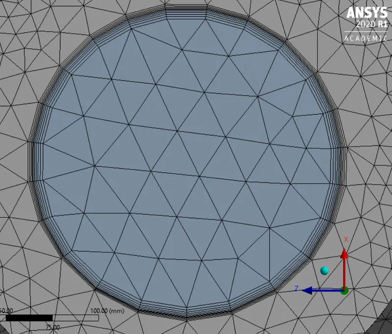
• Number of inflation layers5
• Total thickness 5mm

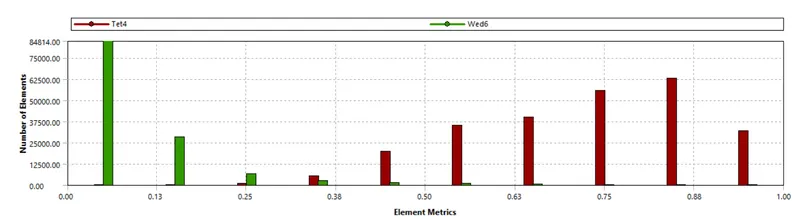
Mesh quality:-

Setup:-

• Here we need to setup a solver. The solver type is pressure based steady state and absolute velocity formation.
• After the solver setup we need to select K-Omega SST turbulence model. K-omega sst model uses K-epsilon model in freestream section of fluid flow and uses K-omega model for the near wall computations. K-omega SST model is good for attaining thermal behaviour near the inner wall.

Boundary conditions:-

• After selecting the viscous model we need to assaign the boundary conditions to different part of component. Since we have already named the parts it automatically selects the boundary conditions.
• for inlet it is velocity inlet with velocity magnitude of 5m/sec and temperature of air is 700K
• for outlet it is pressure outlet with pressure gauge of 0pa.
• for outer wall convection it is thermal convection with heat transfer coefficient of 20 WK/m^2.
• Then we need to initialize the solver with hybrid initialization method and setup the number of iterations.

RESULTS:-

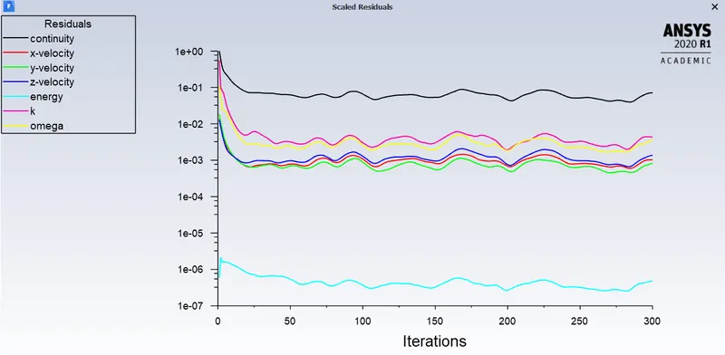
Residuals plot:-

Post processing results:-

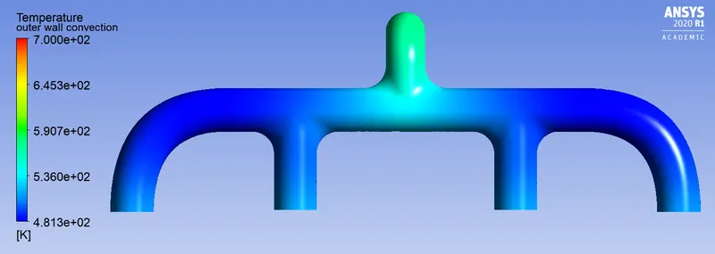
Temperature contour at outer wall:-

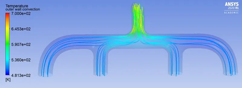
Velocity streamline:-

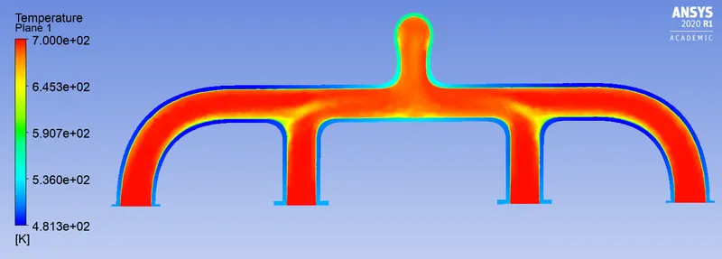
Temperature contour:-

Heat transfer coefficient at outer wall:-

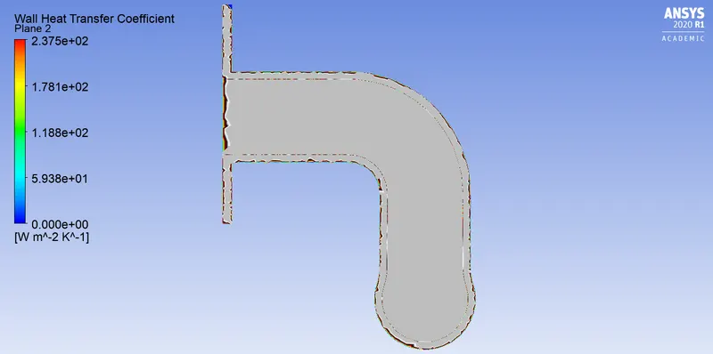
Velocity contour:-

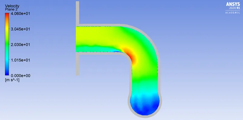
CASE 3:- y+ value 2.6

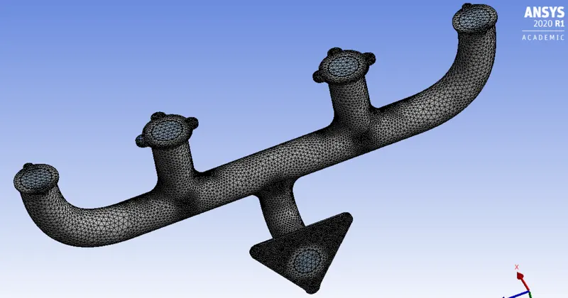
Meshing:-

• Element size 150mm (Fluid domain)
• Body sizing 8mm (outer body)

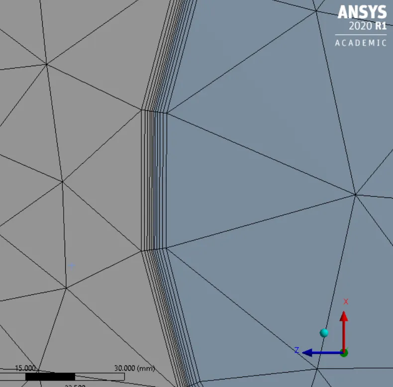
Inflation:-

• Number of inflation layers5
• Total thickness 2mm

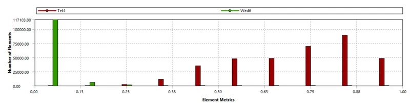
Mesh quality:-

Setup:-

• Here we need to setup a solver. The solver type is pressure based steady state and absolute velocity formation.
• After the solver setup we need to select K-Omega SST turbulence model. K-omega sst model uses K-epsilon model in freestream section of fluid flow and uses K-omega model for the near wall computations. K-omega SST model is good for attaining thermal behaviour near the inner wall.

Boundary conditions:-

• After selecting the viscous model we need to assaign the boundary conditions to different part of component. Since we have already named the parts it automatically selects the boundary conditions.
• for inlet it is velocity inlet with velocity magnitude of 5m/sec and temperature of air is 700K
• for outlet it is pressure outlet with pressure gauge of 0pa.
• for outer wall convection it is thermal convection with heat transfer coefficient of 20 WK/m^2.
• Then we need to initialize the solver with hybrid initialization method and setup the number of iterations.

RESULTS:-

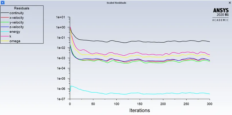
Residuals plot:-

Post processing results:-

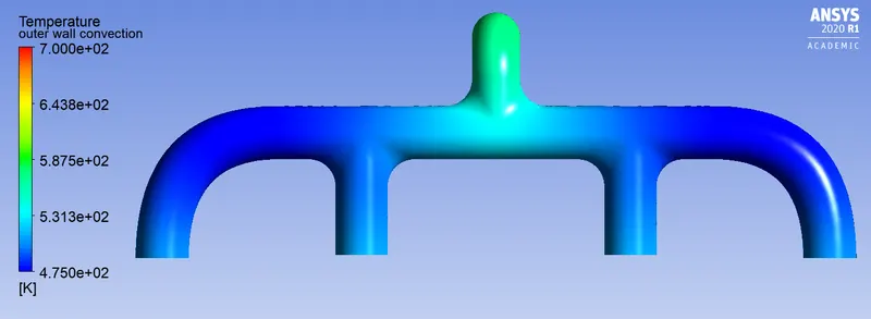
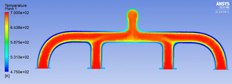
Temperature contour at outer wall:-

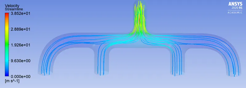
Velocity streamline:-

Temperature contour:-

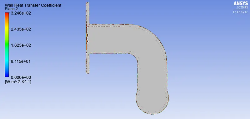
Heat transfer coefficient at outer wall:-

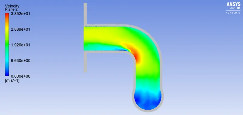
Velocity contour:-

Verification:-

We can verify the simulation results by performing grid independence test or by calculating the nusselts number and heat transfer coefficient.

Where,

• h is heat transfer coefficient of the flow
• L is the length
• K is the thermal conductivity of the fluid
• Nu is the Nusselts number

First we need to find nusselts number this can be found by Dittus Boelter equation.

Where,

• Re is the Reynolds number
• Dh is the Hydraulic diameter
• Pr is the Prandtl number
• Nu is the Nusselts number

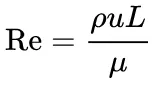
Re= (1.225*5*0.08)/1.7894e-05 =27378

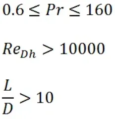
After calculating the nusselts number we can find the heat transfer coefficient.

CONCLUSION:-

• From above results and contour plots we can observe that Refined mesh i.e as the number of elements increases we get more accurate results.
• Value of surface and wall heat transfer coefficient depends on the mesh quality.
• Accuracy of prediction mainly depends on mesh quality, number of elements and inflation layers.
• Mesh need to accurately accommodate the geometry around the curvatures and mesh should be conformal for smooth transfering of mesh in different zones.
• And also the y+ value in the calculation of 1st layer thickness plays a important role.