Week 5 - Rayleigh Taylor Instability
Aim:
An analysis of the Rayleigh Taylor wave simulation for different mesh sizes, its effects on CFD, and a comparison of simulations and analytical methods Define the Atwool Number and discuss its research and application in various scenarios.
Introduction:
- The Rayleigh–Taylor instability is an instability of an interface between two fluids of different densities that occurs when the lighter fluid is pushing the heavier fluid and the potential energy of the configuration is lower than it was in the initial state. This instability can be thought of as an example of a phase transition. Therefore, the disturbance will worsen, which will result in a further release of potential energy. This will occur because the material with a higher density will fall under the influence of the (effective) gravitational field, while the material with a lower density will be further displaced upwards.
- The first sign of instability is the formation of mushroom-like spikes, which are followed by the formation of bubbles over the volume of denser fluid and spikes in the volume of lighter fluid. Next, turbulent mixing takes place with the formation of eddy formations, and finally, chaotic mixing takes place, which leaves denser fluid at the bottom and lighter fluid at the top.
- The importance of the Rayleigh-Taylor instability may be seen anywhere denser and lighter materials combine as a result of natural forces like gravity, beginning with basic items found in everyday life and progressing all the way up to galaxies in the universe. One such example is the oil spill that occurred across the oceans, and another is the crab nebula that occurred in space.
Methodologies for Solving and Modeling:
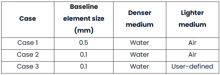
- We are going to solve for the three cases that were mentioned in Aim.
- We will be creating the geometry and performing structured quads CFD mesh using ANSYS Fluent solver. After that, we will set up the physics of fluid flow and run the iterations to get solutions. Finally, we will use post processing to interpret the data in the form of plots, contours, vectors, streamlines, and so on.
- We will examine grid independence for the Rayleigh Taylor instability study using gravity on of -9.81 m/s2 and the laminar viscous model. When we talk about the grid independence study, we mean that we are going to look at 2 different scenarios.
- Because we are working with a student edition of ASNYS, we will be restricted in the number of variables we may experiment with. Then, to ensure the simulation is accurate, we compile a database of the case study's findings and compare them to those found in publicly available literature or published book data.
Preprocessing and Solver setting:
Let's launch the ANSYS workstation right now. You can either double click on the Fluent button or use the drag-and-drop feature in the schematic window to create fluid flow. Steps like
GEOMETRY > MESH > SETUP > SOLUTION > RESULTS
make up the streamlined procedure. Before moving on to the next phase, you will need to finish each step in its entirety.
Case 1 will be discussed in depth in the grid independence study.
GEOMETRY >
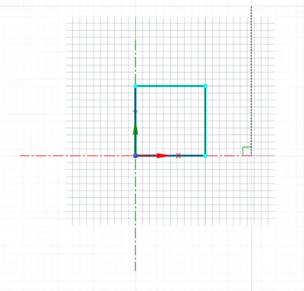
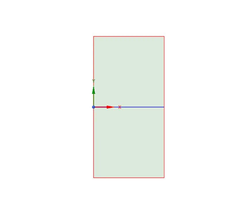
To create a new SpaceClaim Geometry in the Fluent, right-click on the Geometry icon, and then select the option. Once the application for space claim has been opened, choose the New sketch option, and then move the mouse pointer to the upper right corner so that the XY plane may be selected. The square will have sides that are 20 millimetres long, and using the Pull tool or Return to 3D should change the 2D sketch into a plane. We are going to make another plane just like this one using a new component. During the meshing process, we are going to make use of SHARE TOPOLOGY so that the nodes can be shared.
We are all set to go at this point. As soon as the geometry is available, we are able to close the space claim and verify that the fluid flow geometry has been changed, as indicated by a green tick.
MESH >
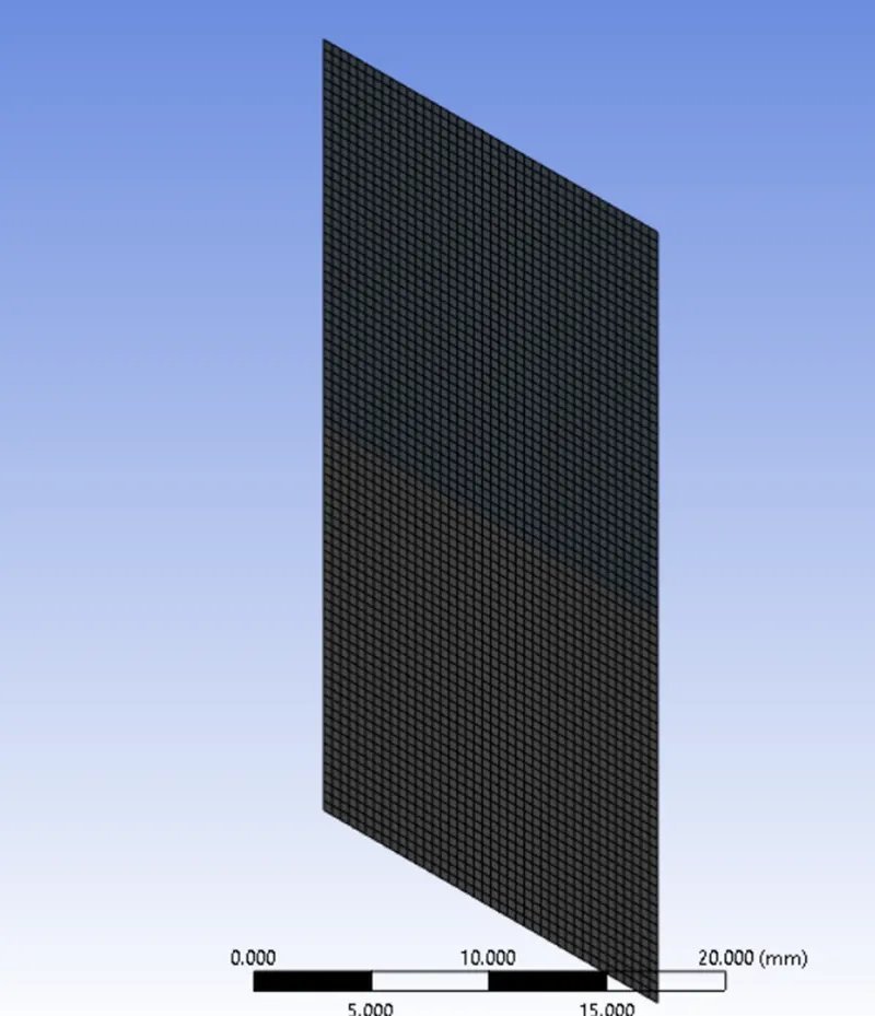
- The Mesh window can be accessed by right-clicking on it and selecting "edit." When you click the GENERATE MESH button in the Mesh window, a mesh will be generated automatically based on the geometry we've already worked on.
- If you want to do a study at 0.5 mm resolution but the default base mesh is 10 mm, you can do it by navigating to the mesh details page and making the necessary adjustments there. A total of 3200 elements are available with a mesh size of 0.5 mm.
- For any modifications, the mesh information must be updated by clicking the update icon, or a lightning bolt symbol will appear to remind the user to do so.
- We are going to give the faces in the air and water domains names like Air and Water by choosing the faces, then using the 'N' button to give them names after naming them. When this is finished, we should notice a green tick somewhere close to Mesh. It is possible for us to shut the mesh window.
SETUP >
- When you right-click on the Setup icon, the Fluent launcher will appear. Select 3D, Double precision, and the amount of cores according to the user's system settings before clicking on the start button in the Fluent launcher.
- Upon opening, there are a few decisions that need to be made in order to create the simulation definitions. We are going to select Type: Pressure based, and then we are going to select Pressure based. Formulation of velocity is absolute, while time is transient. We have the option to pick laminar flow in addition to turning on viscous under the Physics tab. In the Y direction, set the acceleration to -9.81 m/s2 and activate gravity.
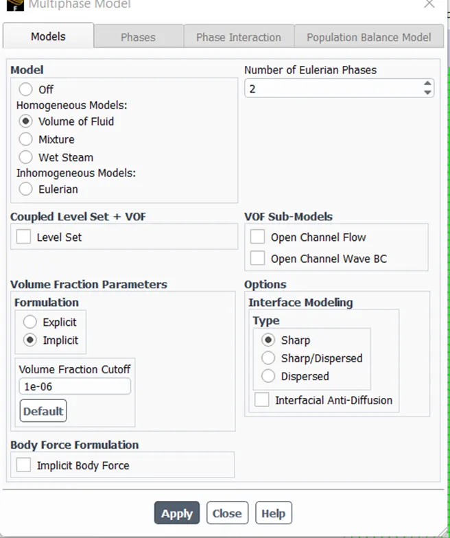
- Simply pick the VOF method, implicit, and then choose air as the primary phase after clicking on the Multiphase tab.
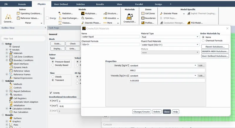
- In the section labelled "Materials," we will make air the default material, and we will set the material type to "Fluid."
SETUP >
When you right-click on the Setup icon, the Fluent launcher will appear. Select 3D, Double precision, and the amount of cores according to the user's system settings before clicking on the start button in the Fluent launcher.
Upon opening, there are a few decisions that need to be made in order to create the simulation definitions. We are going to select Type: Pressure based, and then we are going to select Pressure based. Formulation of velocity is absolute, while time is transient. We have the option to pick laminar flow in addition to turning on viscous under the Physics tab. In the Y direction, set the acceleration to -9.81 m/s2 and activate gravity.
Simply pick the VOF method, implicit, and then choose air as the primary phase after clicking on the Multiphase tab.
In the section labelled "Materials," we will make air the default material, and we will set the material type to "Fluid." With the help of the Fluent database, we'll be able to incorporate water.
Choose the air for the air domain, and water for the water domain, according to the conditions of the cell zone.
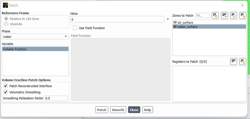
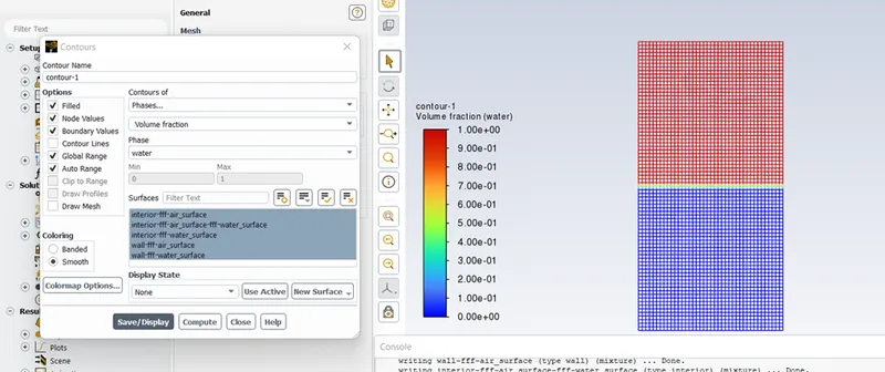
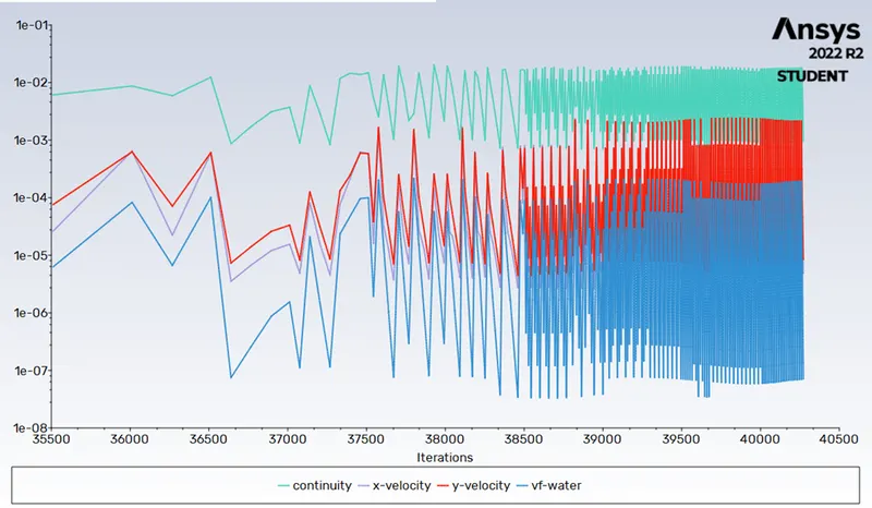
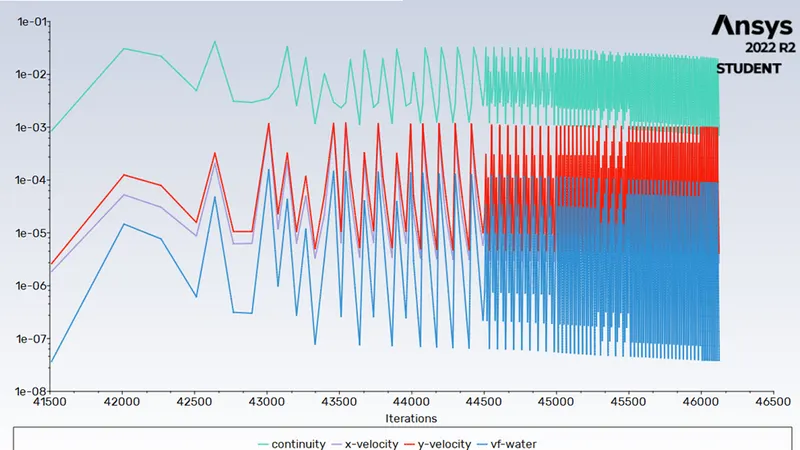
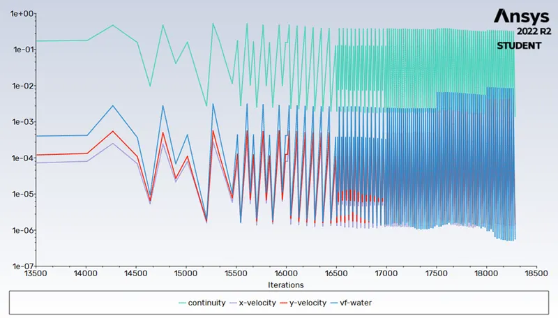
Now is the appropriate time to initiate the simulation. To begin the simulation for the physics that have been set up above, we must first initialise the entire flow field by clicking on the t=0 initialise icon. This will allow us to start the simulation. In order to solve problems involving many phases, we need to use the Patch programme, set the input value for air to zero, and set the input value for water to one. The timestep can be set to 0.002 seconds in the Run Calculation section, and the number of time steps can be set to 2500. This will give us a time interval of 5 seconds. Using Autosave will save contours snippets at time intervals, and we can create an animation in post processing. Clicking on the Calculate button will begin the iterations. Following the iterations, the scaled residuals phase contour is obtained. New phases have been added to the phase contour in the results page under Graphics > Contours. Simply double clicking on the scale will bring up the editing options.
If you are viewing the simulation reports in the Outline view, clicking on the Report Outline > Generate button should produce an Ansys Fluent Simulation Report. This report is automatically generated and contains all of the information regarding the simulation. Additionally, a PDF version of this can be generated. Since we are through with the setup, you may now close it.
- Choose the air for the air domain, and water for the water domain, according to the conditions of the cell zone.
- Now is the appropriate time to initiate the simulation. To begin the simulation for the physics that have been set up above, we must first initialise the entire flow field by clicking on the t=0 initialise icon. This will allow us to start the simulation. In order to solve problems involving many phases, we need to use the Patch programme, set the input value for air to zero, and set the input value for water to one. The timestep can be set to 0.002 seconds in the Run Calculation section, and the number of time steps can be set to 2500. This will give us a time interval of 5 seconds. Using Autosave will save contours snippets at time intervals, and we can create an animation in post processing. Clicking on the Calculate button will begin the iterations. Following the iterations, the scaled residuals phase contour is obtained. New phases have been added to the phase contour in the results page under Graphics > Contours. Simply double clicking on the scale will bring up the editing options.
- If you are viewing the simulation reports in the Outline view, clicking on the Report Outline > Generate button should produce an Ansys Fluent Simulation Report. This report is automatically generated and contains all of the information regarding the simulation. Additionally, a PDF version of this can be generated. Since we are through with the setup, you may now close it.
 |
 |
 |
 |
SOLUTION >
It's possible to see the green checks in both the setup and the solution since some solution is calculated during the setup phase.
RESULTS >
If you click the Results with the right mouse button, the Post processor should open. The default view of the model is a wireframe, and we can make a plane in the XY plane to observe contours. In a manner analogous to that of setup and solution, all plots and contours can be generated in this section. Furthermore, we have the ability to generate an animation of the velocity contour by first clicking on AUTOSAVE during the solution, then clicking on ANIMATE, and finally selecting the make movie option before saving the file in the location of our choosing.
For Case 2, we will carry out the same steps as before, with the exception that the grid size will be adjusted during the meshing stage. We need only make a DUPLICATE of the case 1 fluent file in order to make any necessary edits.
In the third scenario, the user-defined material will have a density of 400 kg/m3 and a viscosity of 0.001 kg/ms, which will be entered under materials.
RESULTS:
Following the execution of the same simulation methods across all of the cases derived from aim, we now have a number of data that can be compared and investigated. We are going to organise all of the contours and animations so that we can examine them side by side and reach a decision. Only the outcomes of all of the examples are shown here; the inferences and interpretations based on those results will be briefly reviewed before the conclusion.
Case 1: Coarse mesh (0.5 mm) - Air and Water
Residual plot
Animation link
Case 2: Fine mesh (0.1 mm) - Air and Water
Residual plot
Animation link
Case 3: Fine mesh (0.1 mm) - User defined material and Water
Residual plot
Animation link
CONCLUSION:
- According to what is stated in Rayeligh's Taylor, the fluid with a higher density will sink, whereas the fluid with a lower density will float to the surface. Because water is the heavier fluid in all three scenarios, it is easy to see the process taking place in all three of them. Important aspects to keep in mind across all simulations are the following:
- When the mesh size is reduced, the quality of the fluids that are submerged improves and becomes more accurate.
- On the other hand, the more detailed the mesh, the longer the computation time will be.
- In the third scenario, we changed the properties, and because the fluid was denser than air, the mixing process had to be different than in the previous two scenarios.
- In the third scenario, the layer of fluids was produced as a result of denser fluids submerging, as can be seen in the example of oil and water. In the early stages, we were able to observe the formation of layers as well as bubbles as a result of gravitational pull. However, a denser fluid and a fluid with a high viscosity were the reasons for this.
- If the primary fluid were more dense than water, then we would not observe any movement in the fluid at all.
The Atwood index:
The atwood number is a dimensionless number that is employed in the research of hydrodynamic instabilities in density stratified flows. It is found in the field of fluid dynamics. It is a density ratio, and its definition is as
A= ρ1−ρ2ρ1+ρ2
where
ρ1
= density of heavier liquid
ρ2
= density of lighter fluid
FOR CASE 1 &2
ρ1
= 998.2kgm3
(water)
ρ2
= 1.225 kgm3
(air)
A= 998.2 - 1.225/998.2+1.225
A= 0.997
FOR CASE 3
ρ1
= 998.2kgm3
(water)
ρ2
= 400 kgm3
(air)
A= 998.2-400/998.2+400
A= 0.427
Inferences:
We can see that when the density gap between the medias widens, the Atwood number moves closer and closer to one. This is the case for density gaps that are quite small. The value of Atwood is rather near to 0. This is a clear indicator of how quickly the instability spread, as well as the amount of time it took for the mixture to settle once it was mixed. In instance 3, we notice more of symmetric mushroom and spikes, numerous vortices, and the turbulence of mixing takes longer time to settle, however in cases 1 and 2, we see huge mushroom and spike and few vortices as well. This is because case 3 has a smaller Atwood number than case 1 and case 2.