Week 5 - Rayleigh Taylor Instability

Week 5 - Rayleigh Taylor Instability.

Aim:

To simulate Rayleigh Taylor instability phenomena using CFD simulation tool, and study the stages of evolution of instability, use water and air for grid independent study, also use a user defined material and study the instability along with water. Also, we shall be discussing the Atwood numbers for all 3 cases.

Introduction:

The Rayleigh–Taylor instability, is an instability of an interface between two fluids of different densities which occurs when the lighter fluid is pushing the heavier fluid, the potential energy of the configuration is lower than the initial state. Thus the disturbance will grow and lead to a further release of potential energy, as the denser material moves down under the (effective) gravitational field, and the less dense material is further displaced upwards.

Initial instability is visible in formation of mushroom like spikes, which forms bubbles over the denser fluid volume and spikes in the lighter fluid volume, and now turbulent mixing occurs with eddy formations, at last chaotic mixing occurs leaving denser fluid at bottom with lighter fluid at top.

The importance of the Rayleigh Taylor instability is seen wherever denser and lighter mediums mix due to natural forces like gravity, starting from simple everyday objects to galaxies in universe. one such example is oil spillage over oceans and crab nebula in space.

Solving and Modeling approach:

We shall solve for 3 cases as discussed in Aim.We will be using ANSYS Fluent solver to create the geometry and perform structured quads CFD mesh, setup the physics of fluid flow and run the iterations to get solutions, using post processing to interpret the data in form of plots,contours, vectors, streamlines etc.,

With gravity on of -9.81 m/s^2 and laminar viscous model we shall study grid independence for Rayleigh Taylor instability study. When we say grid independence study we shall study for 2 cases as follows.

Case	Baseline element size (mm)	Denser medium	Lighter medium
Case 1	0.5	Water	Air
Case 2	0.1	Water	Air
Case 3	0.1	Water	User-defined

We shall keep in mind we are using a student version of ASNYS, so we are limited with the number of elements to play with. Then, we tabulate the case study results and compare it with the open literature or book data results to validate the simulation.

Preprocessing and Solver setting:

Let us open ANSYS workbench, now opening Fluent flow can be done by drag and drop in the schematic window or by double clicking on Fluent. The fluent workflow is in a series of steps such as GEOMETRY > MESH > SETUP > SOLUTION > RESULTS. Each step has to be completed for the next step to initialize.

In the grid independence study we shall consider case 1 and discuss in detail,

GEOMETRY >

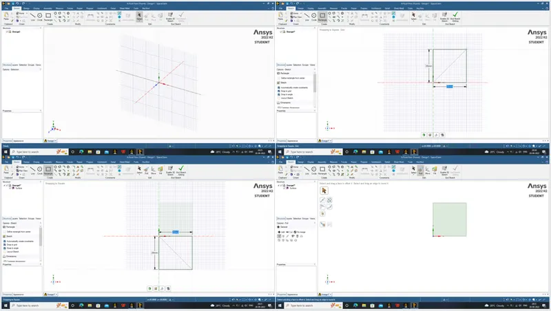
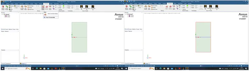
In the Fluent, right click on the Geometry and select New SpaceClaim Geometry. The space claim application opens, select New sketch and moving the mouse pointer to the top right, we can select the XY plane. We shall sketch a square with side 20 mm, Pull tool or Return to 3D should make the 2D sketch into a plane. We shall create another plane like this with New component. We shall use SHARE TOPOLOGY so that the nodes are shared during meshing process

We are good to go now. Once the geometry is ready, we can close space claim and check that the fluid flow (fluent) geometry is updated indicated by a green tick.

MESH >

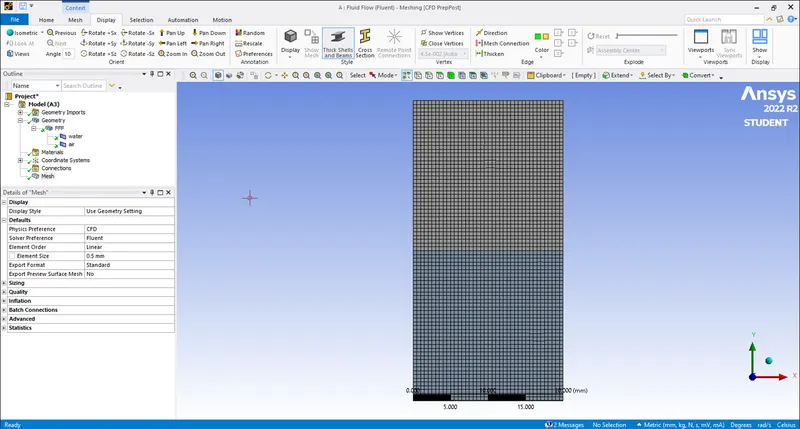
Right clicking on the Mesh and selecting edit opens the Mesh window. Mesh window is preloaded with the geometry we have worked on earlier, so clicking on the GENERATE MESH should create a mesh automatically.

The baseline mesh here by default will be around 10 mm, but we are interested in study of 0.5 mm, we can directly change the mesh size in mesh details tab. For 0.5 mm mesh size, we get 3200 elements.

Any changes made, click on the update icon to update the mesh details or else there is an indication of a thunderbolt sign asking the user to update.

We shall name the air and water domains surfaces such as Air and water by selecting the faces and using the ‘N’ button and name them. Once this is done, we should see a green tick near Mesh. we can close the mesh window.

SETUP >

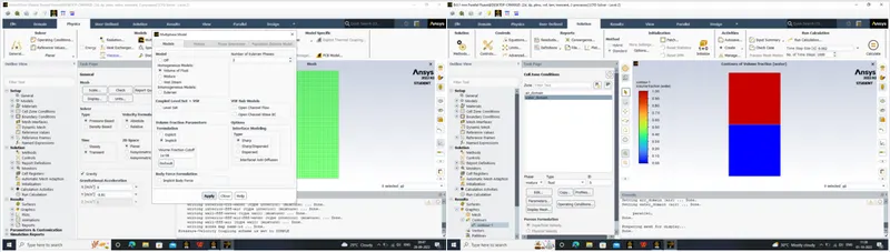
Right clicking on the Setup, opens the Fluent launcher. In the Fluent launcher select 3D, Double precision and select the number of cores as per the user system configuration and click on start.

Upon opening, there are some selections to be done to define the simulation definitions, we shall select Type: Pressure based, Velocity Formulation: Absolute, Time: Transient. Under the Physics tab, we can turn on viscous and select laminar as well. Turn on gravity and set -9.81 m/s^2 in Y direction.

Click on the Multiphase > select VOF method, implicit, and select phases air as primary phase.

Under the materials we shall select air as our default material with material type as fluid. We shall add water from the Fluent database.

Under the cell zone conditions, select the air for air domain and water for water domain.

Now, it's time to start the simulation. In order to start the simulation for the above set up physics, we need to initialize the entire flow field by clicking on the t=0 initialize icon. For Multiphase problems, we need to do Patch, select air and input as 0, and select water and input as 1. In the Run Calculation we can input the timestep as 0.002 s and no of time step as 2500 , so that we get a 5 second, using Autosave saves contours snippets at time intervals and we can create an animation in post processing, and clicking on the Calculate should start the iterations. After iterations, we get scaled residuals phase contour Results > Graphics > Contours > New phases for phase contour. The scale can be edited by double clicking on it.

In the Outline view under Simulation Reports, clicking on the Report Outline > Generate should generate a Ansys Fluent Simulation Report which is automatically generated with all the information of the simulation in it. This can be exported as a PDF also. We are done with setup, we can close the setup.

SOLUTION >

Since some solution is calculated in the setup itself, we can see the green ticks in both setup and solution too.

RESULTS >

Right clicking on the Results should open the Post processor. Default view is a wireframe model, we can create a plane in XY to view contours. Similar to setup and solution, all contours and plots can be created here, in addition to that we can create an animation of the velocity contour by clicking on AUTOSAVE during the solution and clicking on ANIMATE select make movie and save in desired location.

For Case 2, we shall repeat the same except for changing the grid size in meshing step. We can simply DUPLICATE case 1 fluent file and edit in it.

For case 3; under materials we shall input user defined material with density 400 Kg/m^3 and viscosity 0.001 Kg/ms.

RESULTS:

After repeating the similar manner of simulation procedures for all cases from aim, we have a handful of data to compare and study. We shall put in order all the contours and animations for us to compare and come to a conclusion. Here, only the results of all cases are displayed, its inference and interpretation shall be discussed briefly in conclusion.

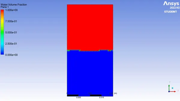
Case 1: Coarse mesh (0.5 mm) - Air and Water

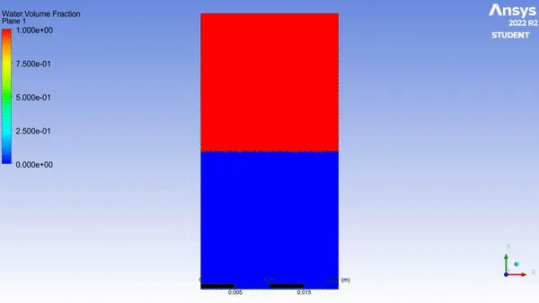
Case 2: Fine mesh (0.1 mm) - Air and Water

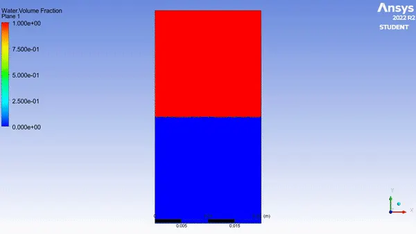
Case 3: Fine mesh (0.1 mm) - User defined material and Water

CONCLUSION:

The comparison between cases 1 and 2 clearly shows that with finer mesh, capturing of the details in instable mushroom and spike formation is very good. For case 3, as the density difference between the two medias decreases, the mixing is much easier and mushroom and spike formations are clearly visible but the settling time is longer.

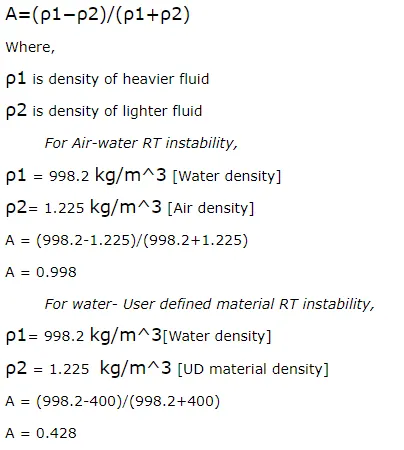
Atwood number:

It is a dimensionless number that is used to study hydrodynamic instabilities in density stratified flows.

Inferences:

We can see that as the density difference between the medias increase, the Atwood number is close to 1 for lower density differencesm Atwood number is close to 0. This is an clear indication of rapidness of the instability, and the time taken to settle after the mixing. for lower Atwood number of 0.428 in case 3, we see more of symmetric mushroom and spikes, many vortices and turbulence of mixing takes longer time to settle, whereas in cases 1 and 2, we see large mushroom and spike and few vortices as well.

References:

https://www.sciencedirect.com/science/article/abs/pii/037015739190153D