Week 5 - Rayleigh Taylor Instability

Aim

Conduct a CFD study on the Rayleigh Taylor Instability using water and air on two different meshes to understand the influence of the mesh on the simulation. Further, substitute air with a user-defined fluid with higher density to understand the influence of the Atwood number on the instability.

Introduction

In a multi-fluid system, small perturbations at the interface of distinct fluids will grow due to the effects caused by buoyancy and shear-driven instabilities. These instabilities will lead to turbulent mixing zones in the form of bubbles and spikes brought by the motion of the light and heavy fluids respectively penetrating into each other. The instabilities can be broadly classified into three types [1]:

1. Rayleigh Taylor Instability:
   
   This instability occurs at the interface of two fluids with varying densities, where the lighter fluid pushes the heavier fluid. Can be seen in the motion of water when suspended above oil and under the effect of gravity.
   
   
2. Richtmyer-Meshkov Instability:
   
   This instability occurs at the interface of two fluids with varying densities where the perturbations are accelerated by a shockwave. Can be seen in supersonic combustion where the fuel-oxidant interface is enhanced by the breakup of the fuel into fine droplets due to this instability.
   
   
3. Kelvin-Helmholtz Instability:
   
   This instability occurs at the interface of two fluids at varying velocities relative to each other. Can be seen in the formation of clouds in the atmosphere.

CFD mixing Models derived from the mathematical analysis of the Rayleigh Taylor Instability:

1. Young's Mix model:
   This is a phenomenological model developed by Young [2] which is derived from the results of direct numerical simulations and experimental data. Unresolved parts of this model are closed by using extra terms of mass, diffusion, drag and turbulent dissipation which are defined by a multitude of relationships and model parameters.
   
   
2. Ensemble-average Microphysical Modelling:
   A version of this type of model was proposed by Glimm et al [3], which performs an ensemble averaging of the Euler equations over infinite microscopic flow realisations.
   
   
3. Hybrid Turbulent Mix Model:
   This model was proposed by Cranfill [4] and is based on the decomposition of the Navier Stokes equations into mean and fluctuating parts. Here the turbulent contributions are divided into ordered and disordered parts where the ordered parts are estimated from the average drift motions produced by a set of multi-fluid interpenetration equations, and the disordered parts are estimated from single-fluid turbulence equations.
   
   
4. Besnard, Harlow, and Rauenzahn Model:
   The Single fluid variable-density turbulence model or otherwise called the BHR model was developed by Besnard et al [5]. This model uses the Reynolds decomposition of the Navier-Stokes equations for a single field with potentially large density variations.
   
   
5. Buoyance Drag Model:
   Various buoyancy drag-based models have been proposed by multiple authors and are used primarily in one-dimensional Rayleigh-Taylor and Richtmyer-Meshkov instabilities [1]. The model describes the dynamic position of the interface of the two fluids which are created by the RT/RM instabilities.
   
   
6. The two-equation KL Transport Model:
   This model was developed by Dimonte et al [6] and is based on the buoyancy drag models. The equations of this model are constructed only with local parameters so that it can be applied to multidimensional flows with multiple shells of materials. The unknown coefficients in this model have been determined by comparing analytical and numerical solutions with the experiments performed on RT/RM instabilities.
   
   

Stages of Rayleigh-Taylor Instability:

The growth of the Rayleigh-Taylor instability can be categorized into various stages [7] :

• Stage 1: This stage describes the initial perturbations caused at the interface of the two fluids and are extremely small in nature.
  
  
• Stage 2: In this stage, the amplitude of the perturbations increases non-linearly and is affected by the value of the Atwood number of the system. The lighter fluid will be seen to move into the heavier fluid in the form of bubbles while the heavier fluid tries to penetrate the lighter fluid in the form of thinner spikes.
  
  
• Stage 3: This stage is characterised by the development of structures on the spikes and the interface among the bubbles which would have originated from several sources combined.
  
  
• Stage 4: The final stage involves the breakup of the spikes and penetrations of the bubbles due to various mechanisms and leads to turbulent chaotic mixing of the two fluids.

Atwood Number:

The Atwood number is a dimensionless number commonly used in the study of hydrodynamic instabilities where fluid motion is dictated primarily by the differences in densities.

`A = (rho_1 - rho_2)/(rho_1 + rho_2)`

where,

`rho_1` - Density of heavier fluid [kg/`m^3`]

`rho_2 ` - Density of lighter fluid [kg/`m^3`]

Courant-Friedrichs-Lewy (CFL) number:

The Courant-Friedrichs-Lewy number, most commonly referred to as CFL number or Courant number, relates the time step size to the interval between spatial coordinates and the maximum speed that information can travel through them. CFL number of 1 implies information will pass through 1 spatial coordinate across each time step. This will usually provide the most accurate solutions however, is computationally expensive. Increasing the CFL number quickens the simulation process and reduces computational costs at the expense of solution accuracy. Estimation of CFL number can be done by:

`CFL = (u Delta t)/(Delta x)`

Where,

u- velocity magnitude at the cell [m/s]

`Delta t` - Time step size [s]

`Delta x` - Interval between spatial coordinates/ Element sizing of the cell [m]

Method

Geometry and Fluid Domain

The geometry to simulate the Rayleigh Taylor Instability was constructed as in the schematic below:

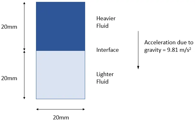
This geometry will be the fluid domain where the upper half will have the heavier fluid and the lower half will have the lighter fluid respectively at t=0. The interface region marked will be the zone where both fluids meet and will be the region where initial perturbations due to instabilities will arise.

Mesh

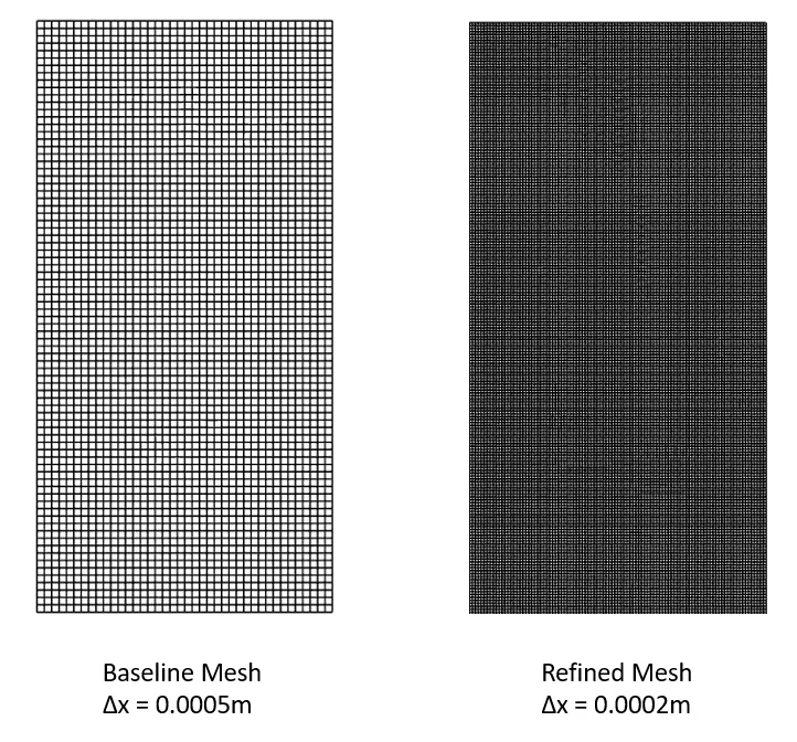
The hex dominant structured mesh type was used for this analysis. The initial mesh was generated with a global element sizing of 5e-4m and contained 3000 mesh cells. The refined mesh was generated with global elements sizing of 2e-4m and contained 20000 mesh cells. Illustrations of the two mesh can be seen below:

Solver and Boundary Conditions

Simulations were performed on Ansys Fluent 2022 R2. In the first analysis, the water and air at their default properties were used as the heavier and lighter fluid respectively. In the second analysis, a user-defined material with density = 400 [kg/`m^3`] and dynamic viscosity = 0.001 [kg/ms] was substituted for air as the lighter fluid.

The unsteady pressure-based solver was used for this analysis. The volume of fluids model was used to model the volume fractions of the two phases and their interactions. The laminar viscous model was used in the analysis as the flow velocity was low and therefore turbulence modelling will not be required.

The acceleration due to gravity was set to -9.81 [m/s^2] in the Y-direction. All bounding walls were set to no-slip condition and the solution was initialized and patched with volume fractions of heavier and lighter fluids in their respective zones.

The adaptive time stepping method was used and run for a maximum of 4.6 flow seconds. The global courant number was kept at 2 as this was deemed sufficiently accurate for the simulation and not as computationally expensive as compared to a CFL 1. The initial time step size was estimated based on the velocities derived from a preliminary simulation to ensure CFL = 2 and shown in the table below:

Simulation Run	Initial Time Step Size
Base Mesh (Air- Water)	0.006 s
Refined Mesh (Air - Water)	0.002 s
Refined Mesh (Air - User-defined Material)	0.002 s

The minimal and maximum time step size increments were kept at the defaults 1e-5 s and 10 s respectively. A maximum of 20 iterations were run for each time step and their convergence was monitored based on scaled residuals of continuity and momentum reaching below 1e-3. The facet-average volume fraction in the air zone was also monitored through the flow time to quantify if the flow has reached a steady state. A contour of volume fractions of the heavier fluid in the domain was also exported in each flow time step to visualise the instability and its development.

Results

Case 1: Baseline Mesh (Air- Water)

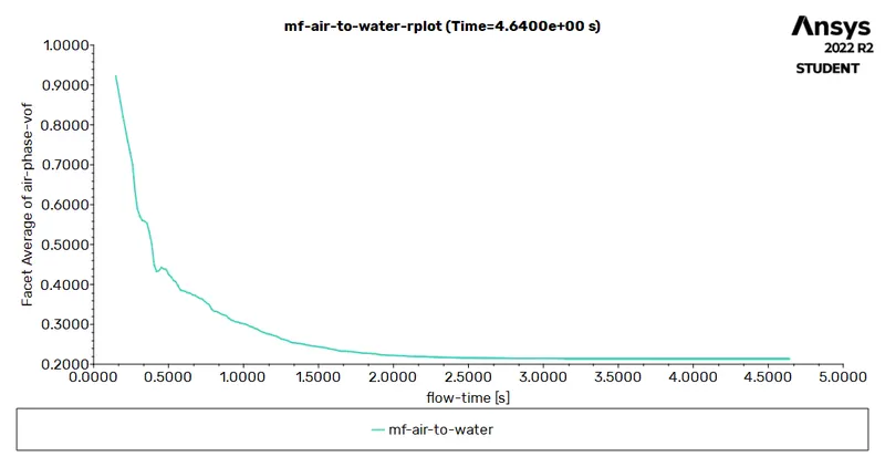
Atwood number A = 0.998

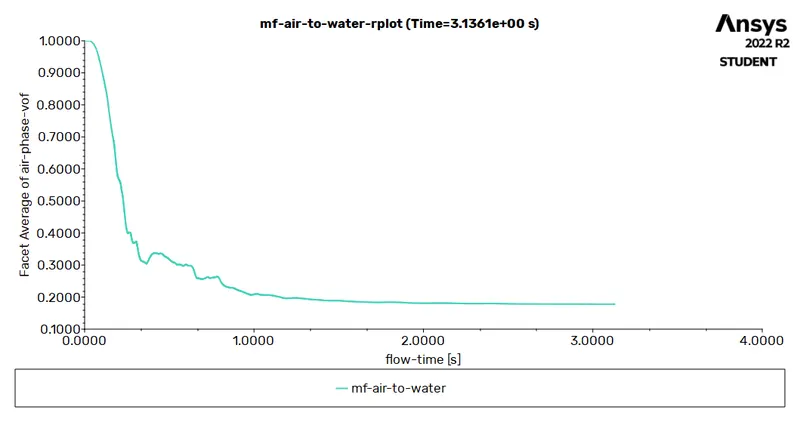
The image below shows the variation of the average volume fraction of air in the lighter fluid zone of the domain across flow time. The volume fraction of air can be seen to stabilise after a certain point and therefore the entire system can be deemed to have reached an equilibrium.

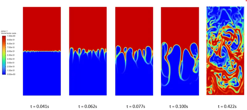
In the image below, the first four contours depict the four stages of the Rayleigh-Taylor instability and the final contour depicts the instance when the heavier fluid reaches the upper boundary of the domain.

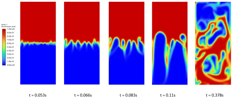
It is evident that the resolution of the contours is poor and the spikes and bubbles seen in this image are pixelated indicating a need for mesh refinement. The solution seen above has captured the major structures of the instability well but however fails to resolve the small-scale structures which are important as the initial perturbations are very small in nature.

Drive Link to full video:

https://drive.google.com/file/d/1cONs6zHxxhgGCIPOZoGiLkb46kQeGV73/view?usp=sharing

Case 2: Refined Mesh (Air- Water)

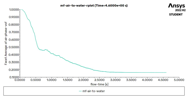
Atwood number A = 0.998

The image below shows the variation of the average volume fraction of air in the lighter fluid zone of the domain across flow time. The volume fraction of air can be seen to stabilise after a certain point and therefore the entire system can be deemed to have reached an equilibrium.

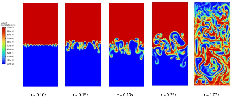
In the image below, the first four contours depict the four stages of the Rayleigh-Taylor instability and the final contour depicts the instance when the heavier fluid reaches the upper boundary of the domain.

It is clear that refining the mesh has removed all the pixelation in the images and the structures seen in this image are well resolved hence the mesh can be deemed to be sufficiently refined.

The various stages of the RT instability can be seen to occur sooner in the refined mesh case compared to the baseline case. This can be attributed to the capability of the mesh to pick up the smallest of perturbations in the domain due to its high mesh resolution. The third stage shows the presence of large bubbles created by the low-density fluid and the small sharp spikes of high-density fluid trying to penetrate the low-density fluid. The fourth stage shows the breakup of the bubbles and disintegration of the spikes which will then slowly lead to the fully turbulent mixing as seen in the final image.

The time taken for the heavier fluid to reach the upper boundary is more in the refined case compared to the baseline case. This can be attributed to the increased amount of small-scale mixing occurring in the refined case which is not present in the baseline case. These small-scale mixing regions take up some of the momentum of the fluid and therefore delay the heavier fluid from reaching the upper boundary.

Drive Link to full video:

https://drive.google.com/file/d/1FiDD96W1Rj-ZPUnIpd5p0cv0XbrZ4IaL/view?usp=sharing

Case 3: Refined Mesh (User Defined Material- Water)

Atwood number A = 0.428

The image below shows the variation of the average volume fraction of air in the lighter fluid zone of the domain across flow time. The volume fraction of air can be seen to stabilise after a certain point and therefore the entire system can be deemed to have reached an equilibrium.

In the image below, the first four contours depict the four stages of the Rayleigh-Taylor instability and the final contour depicts the instance when the heavier fluid reaches the upper boundary of the domain.

The initial instability in the first stage is seen to occur at a much later stage compared to the previous cases. This delay can be attributed to the lower Atwood number of this system. The penetration distance of the fluid across the four stages is also far decreased in this case. Various small structures are seen near the interface region even after longer flow times indicating the momentum in the fluid, in this case, is far lower compared to the previous. All the small-scale structures in this system have been resolved well and therefore the refined mesh generated earlier is valid for this system as well. The final image indicating the time for the heavier fluid to reach the upper boundary is well delayed compared to the previous case and is primarily due to the lack of momentum in the system between the two fluids.

Drive Link to full video:

https://drive.google.com/file/d/1p62UnLtmBeRqr0JaFdDqVPqZ8Hlk1Hh3/view?usp=sharing

Influence of the Atwood number:

As seen in the images and video above, the system with a higher Atwood number has much greater momentum in the fluid since the variation in density is high. This leads to faster development of instabilities and the increased penetration distances of the initial spikes and bubbles created at the interface. The lower Atwood number system has far less momentum compared to the previous one and shows a very slow generation of instabilities and the penetration distance of the spikes and bubbles are far lower.

Viability of a steady-state approach:

As evident from the results above, the Rayleigh - Taylor instability is a highly time-dependent problem and therefore prediction of both spatial and temporal parameters is essential to its study. Using a steady-state approach will time average the results of the simulation and remove the temporal component of the flow making the simulation results unusable. Hence, the use of steady-state simulations is not viable for the study of Rayleigh-Taylor instabilities.

Conclusion

A CFD analysis was done to study the Rayleigh-Taylor instability and its dependency on the mesh and the Atwood number. From the study, it was seen that the coarser mesh was able to resolve the large-scale structures of the instability well but was unable to predict any of the small-scale structures. A refined mesh is, therefore, necessary to resolve these small-scale structures in the instability to have a more accurate prediction of the fluid motion. The Atwood describes the variation in the density of the fluids and is seen to affect the overall momentum in the fluid where high Atwood number shows high momentum in the fluids and low Atwood number shows lower momentum in the fluids. From the results of the simulations, it was also clear steady-state modelling approach of the Rayleigh-Taylor instability will not be viable due to its lack of temporal resolution.

References

1. Baolian Cheng, Review of turbulent mixing models, Acta Mathematica Scientia, Volume 29, Issue 6, 2009, Pages 1703-1720, ISSN 0252-9602, https://doi.org/10.1016/S0252-9602(10)60012-4.
   
   
2. David L. Youngs, Modelling turbulent mixing by Rayleigh-Taylor instability, Physica D: Nonlinear Phenomena, Volume 37, Issues 1–3, 1989, Pages 270-287, ISSN 0167-2789, https://doi.org/10.1016/0167-2789(89)90135-8.
   
   
3. GLIMM, J., SALTZ, D., & SHARP, D. (1999). Two-phase modelling of a fluid mixing layer. Journal of Fluid Mechanics, 378, 119-143. https://doi.org/10.1017/S0022112098003127.
   
   
4. Cranfill, C W. A new multifluid turbulent-mix model. United States. https://doi.org/10.2172/465874
   
   
   
5. Besnard, D., Harlow, F. H., Rauenzahn, R. M., & Zemach, C. Turbulence transport equations for variable-density turbulence and their relationship to two-field models. United States. https://doi.org/10.2172/7271399
   
   
6. Dimonte, Guy & Tipton, Robety. (2006). K-L turbulence model for the self-similar growth of the Rayleigh-Taylor and Richtmyer-Meshkov instabilities. Physics of Fluids - PHYS FLUIDS. 18. https://doi.org/10.1063/1.2219768.
   
   
7. D.H. Sharp, An overview of Rayleigh-Taylor instability, Physica D: Nonlinear Phenomena, Volume 12, Issues 1–3, 1984, Pages 3-18, ISSN 0167-2789, https://doi.org/10.1016/0167-2789(84)90510-4.