Rayleigh Taylor Instability

Introduction

A stratified fluid is a fluid with density variations from one point to other. There are two kinds of stratified fluids. The first kind is where the density change is abrupt, where the graph between altitude and density looks like a downward step. An example of such a case is the interface between the flow of air over water or the flow of fresh water over salt water.

The other kind of stratified fluid is the one where the density change is continuous, where the density altitude graph is a curve. An example of such a case is our atmosphere where the density slowly decreases with an increase in altitude.

In systems with abrupt density variation at the interface-

1. Density below the interface is higher than above
   Consider the example of water in a glass. There is a sharp interface between water and air. When this system is disturbed, we see that the interface is no longer a straight line, but a 3-Dimensional wave called a gravity wave. With time, this wave settles down due to gravity and friction making the interface stable and straight again.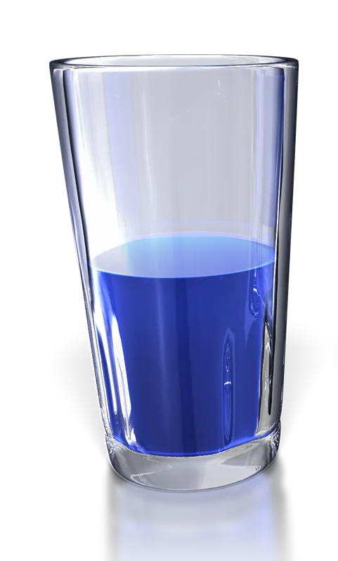
   
   
2. Density below the interface is lower than above
   
   Now, consider a case where the denser fluid is at the top and the lighter fluid. Though this seems illogical, this case does exist and can be visualized with just paper and a couple of glasses. Take a half-filled glass of water and place a stiff paper over its open rim and invert the glass while holding the paper in place. Put this set-up on the opening of another glass. The moment you remove the paper, the case under study is observed. For a microsecond or so, the interface between water and air is perfectly straight and easily distinguishable.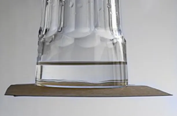
   
   

For further understanding of the stratified flows and their behavior, watch this classic lecture by Robert R.Long from The Jhon Hopkins University.

But what happens after the micro-second? That is our concern in this project.

Due to variations in density, and the difference in the force of gravity on these differential fluids, the interface quickly deforms and becomes highly unstable. This instability of the interface and its behavior is termed the Rayleigh-Taylor instability. Since the heavier mass is displaced and is moved to the bottom, the potential energy of the system is reduced in the process, leading to further reduction of the potential energy until all of the heavier fluid is settled.

Evolution of Rayleigh-Taylor instability

The disturbances initially grow linearly and then non-linearly eventually developing into structures known as plumes and spikes.

The evolution of the RTI follows four main stages. In the first stage, the perturbation amplitudes are small when compared to their wavelengths, and the equations of motion can be linearized, resulting in exponential instability growth. In the early portion of this stage, a sinusoidal initial perturbation retains its sinusoidal shape. However, after the end of this first stage, when non-linear effects begin to appear, one observes the beginnings of the formation of the ubiquitous mushroom-shaped spikes (fluid structures of heavy fluid growing into light fluid) and bubbles (fluid structures of light fluid growing into heavy fluid). The growth of the mushroom structures continues in the second stage and can be modeled using buoyancy drag models, resulting in a growth rate that is approximately constant in time. At this point, nonlinear terms in the equations of motion can no longer be ignored. The spikes and bubbles then begin to interact with one another in the third stage. Bubble merging takes place, where the nonlinear interaction of mode coupling acts to combine smaller spikes and bubbles to produce larger ones. Also, bubble competition takes place, where spikes and bubbles of smaller wavelengths that have become saturated are enveloped by larger ones that have not yet saturated. This eventually develops into a region of turbulent mixing, which is the fourth and final stage in the evolution. It is generally assumed that the mixing region that finally develops is self-similar and turbulent, provided that the Reynolds number is sufficiently large.

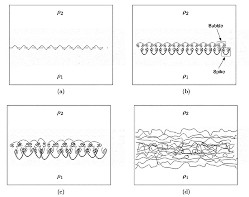
The type of non-linear growth depends upon the density variation between the heavier and lighter fluid. A better indication of this is given by a dimensionless number called as Atwood number which is the ratio of the absolute difference of the fluid densities to their sum.

For an Atwood number close to 0, the instability takes the form of symmetric "spikes" of fluid and for an Atwood number close to 1, the much lighter fluid below the heavier fluid takes the form of larger bubble-like “plumes”

CFD Modelling

There are many models for the instability in focus. Ansys has 3 kinds of them. The VOF model, the Mixture model, and the Eulerian model. In a sense, the VOF and the mixture model are simplified, Eulerian models. The Eulerian model solves the equations for each phase and thus is more complex and expensive than the simplified Eulerian models. For understanding how these models work, please watch the following video by Fluid Mechanics 101.

Geometry creation

Lower plate – 20*20 mm
Upper plate – 20*20 mm
Share topology for conformal meshing

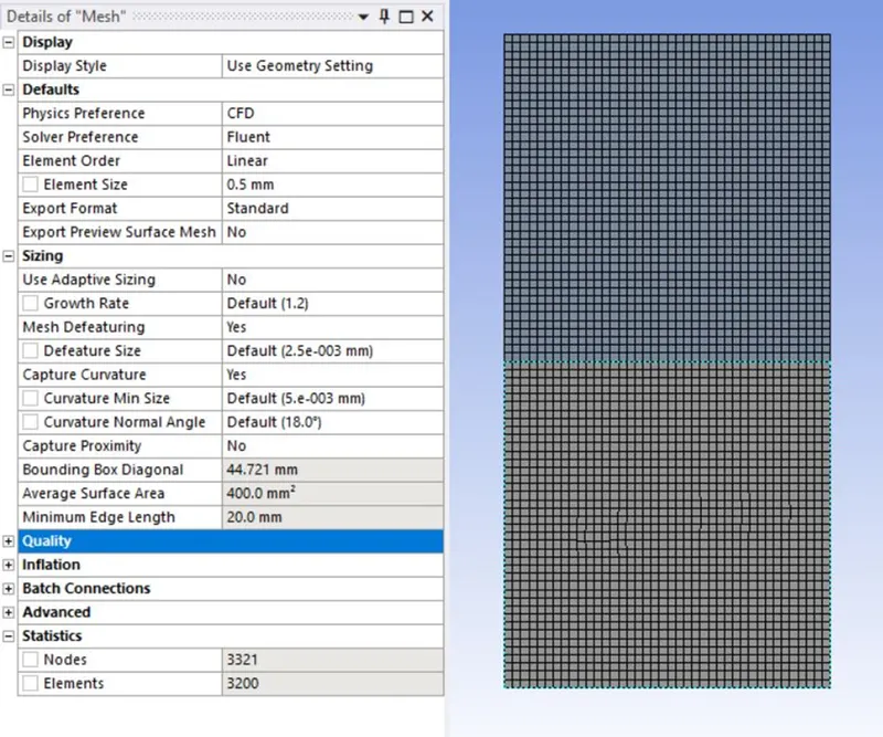
Meshing

Set-up

• Solver - Pressure based (Incompressible flow)
• Energy - Untick (Temperature not desired in this project)
• Gravity - 9.8m/s^2 in the desired direction
• Viscous - Laminar (Free fall under gravity, low velocity, mostly laminar; though the mixing can soon develop into turbulent)
• Multiphase - VOF (Implicit)
• Time - Transient
• Timestep size - 0.025
• Fixed time step Method
• Pressure-velocity coupler - SIMPLE

Results

Note - The gif below has been slowed down for visualisation aid.

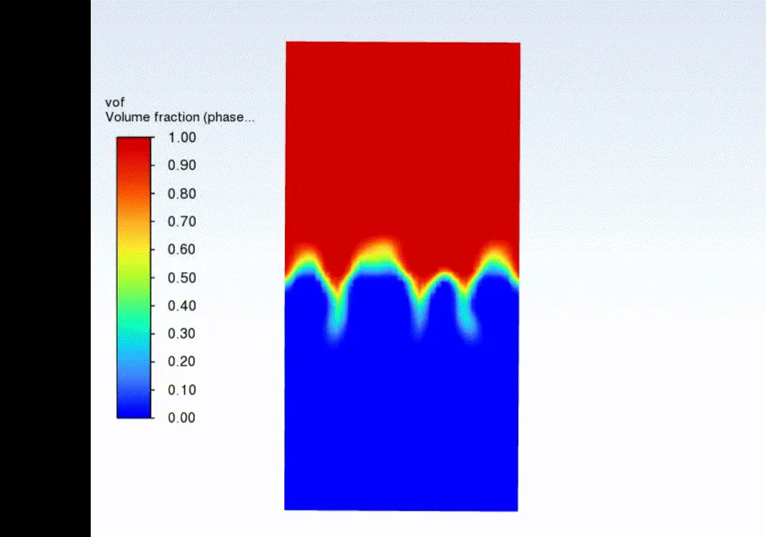
Let’s try to understand what is happening here. Almost instantly, at the center of the region, a large balloon of air moves upwards, making fluid fall right next to it, which looks like a knife-like structure. In fluid mechanics terminology, these are called bubbles and spikes respectively. It is also noticeable that as soon as the initial spikes touch the bottom, more fluid touches the bottom at the walls. This, I assume is due to the surface tension and viscosity between the fluid and wall. But, counter-intuitively, we have not specified any wall condition while setting up, so this might just be symmetry. I would go with the first explanation.

One can easily observe the grids/cells in the above simulation (the simulation is slowed down for easy visualization). This means that the Mesh is coarse in nature and requires refinement.

Re-Meshing

Element size – 0.1mm, i.e., 5 times more refined than the previous case.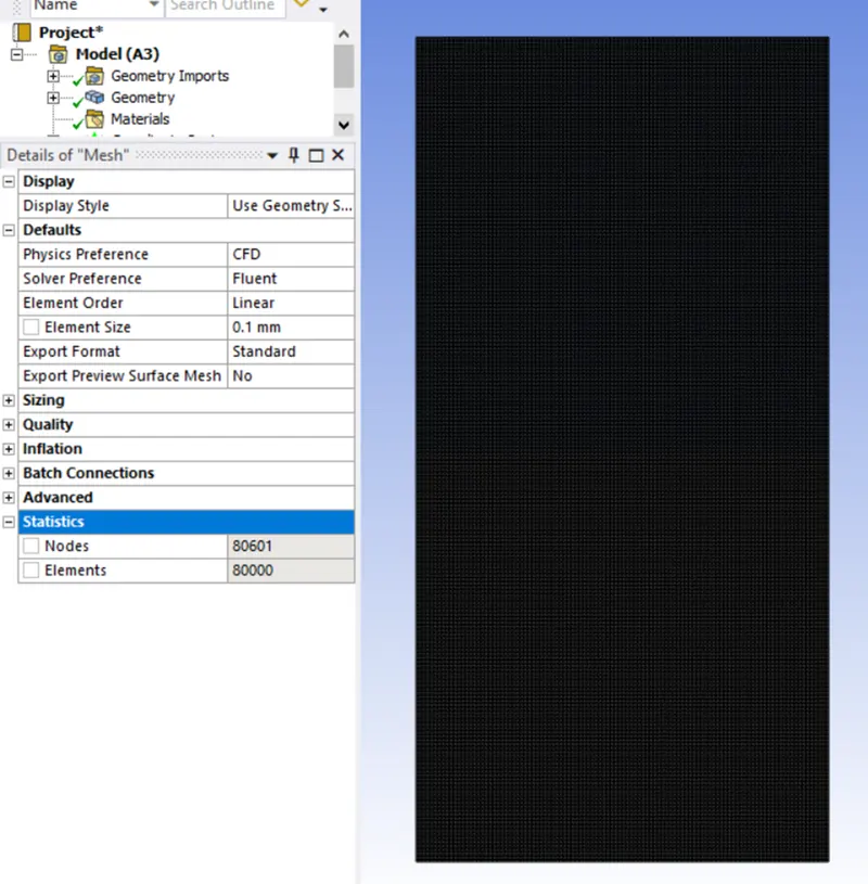

Re-Run

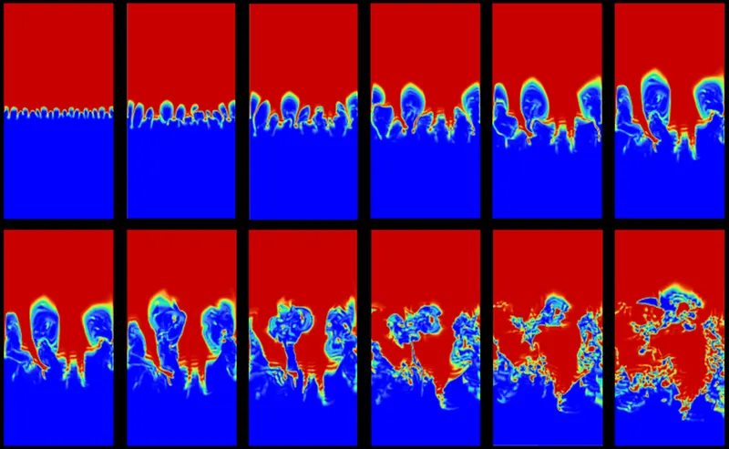
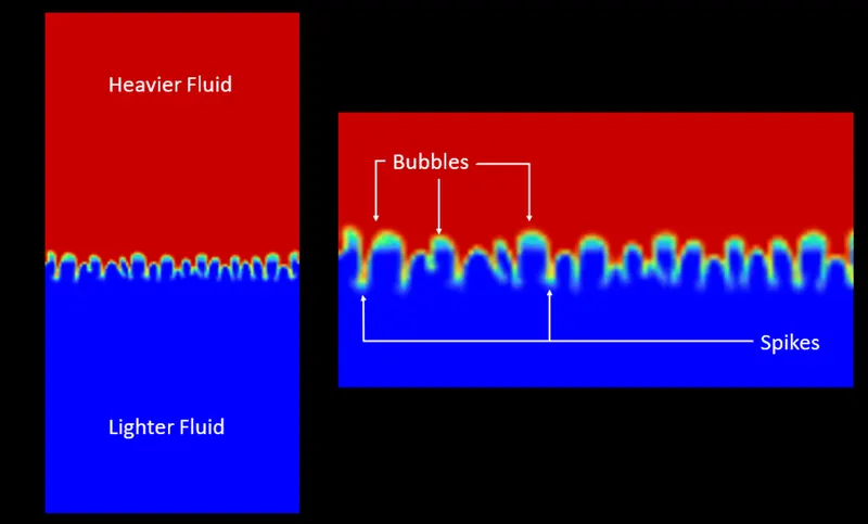
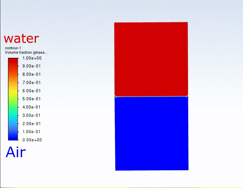
From the above pictures, it can be observed that it is not a single bubble that forms at the center, but rather a lot of balloons and spikes form initially and then grow further to merge and become bigger balloons which break apart and give rise to turbulent mixing.

Unfortunately, the residuals jumped up here and the processor threw a floating-point error implying divergence.

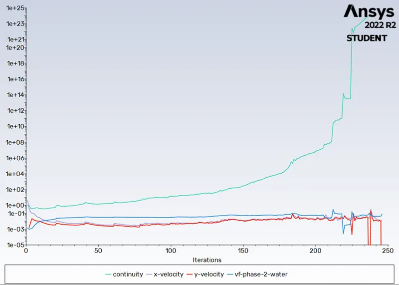
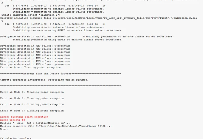
Since divergence was observed, the pressure velocity coupler was changed from SIMPLE to COUPLE method, considering that COUPLE is a good method to avoid divergence. But, even under such condition, divergence was observed.

This problem was overcome by reducing the relaxation factor for COUPLE to 0.35 and limiting the Courant number to 5.
Fixed time step method with timestep size of 0.005 was used to obtain the following results. Alternatively, an adaptive time step method can also be used to obtain similar results. For more information on adaptive time step methods, check https://www.afs.enea.it/project/neptunius/docs/fluent/html/ug/node808.htm

The simulation was made to run for a good 2-3 hrs. before stopping it forcefully to avoid high computational power. The obtained results are good enough to understand the underlying physics.

Note - The gif below has been slowed down for visualisation aid.

case 2 - Water and user denfined material

• User defined material properties :
• Density = 400kg/m3
• Viscosity = 0.001kg/ms

<--- Could not upload the file here due to techncial glitches, will ad it in the comments section --->

In this case, there is not much fluctuation in the interface between the varying density fluids when compared to the previous case. It can also be observed that in the second case, the bubbles and spikes quickly dispersed when compared to the previous cases. This is because of the relation between the densities of these two fluids. This relationship can be better understood using a dimensionless number called Atwood number.

Atwood number

`At=(rho_h-rho_l)/(rho_h+rho_l`

where,

subscript h and l mean heavy and light respectively.

In case 1, where the fluids at study where water and air, the Atwood number is 0.9975

In case 2, where the fluids at study are water and user defined material, the Atwood number is 0.4278

For large density variations, the Atwood number tends to 1 and for small density variations it tends to 0.

If Atwood number is closer to 1, then large bubbles and spikes are formed with greater penetration.