Week 5 - Rayleigh Taylor Instability

AIM:

The aim of this study is to simulate the Rayleigh-Taylor Instability(RTI) with 2 different meshes and 2 different sets of Fluids. Draw inferences from the simulation and give a brief overview of RTI, its significance and practical applications.

INTRODUCTION:

Rayleigh-Taylor Instability(RTI) also called RT Instability, is the instability of the interface of 2 fluids of different densities, where the lighter fluid pushes the heavier fluid. RTI takes place at very large scales such as Interstellar Bodies and even on microscopic scales such as nuclear fusion, which is why its study is substantial.

It also plays a vital role in affecting Earth's climate, such as evaporation of the ocean surface which makes the top layer saltier and heavier.

CFD models based on mathematical analysis of Rayleigh Taylor waves:

Mass diffusion model:

The mass diffusion equation, which is what actually causes mixing in the fluids, specifies how mass and energy are transported due to model viscosity. Though the viscosity is high enough, the diffusion process may nevertheless result in significant mixing even if all configurations are Rayleigh Taylor unstable.

Single fluid models:

• Potential flow model: This model is applicable to all stages of instability changes, from linear through early nonlinear to asymptotic, although it is only applicable when Atwood number = 1. The flow equations in this model are expanded to second-order around the bubble tips by single-mode perturbation, yielding an ordinary differential equation for the bubble velocity.
• Buoyancy drag model: It is applicable to all Atwood numbers but is only effective during the non-linear instability stages. The breadth of the mixing layer is changed using ordinary differential equations. By balancing the effects of drag, buoyancy, and inertia, the amplitudes of the bubbles or spikes are specified. These models typically do not account for demixing, also known as counter gradient transfer, which is the lowering of total fluid masses within the mixing zone. They are also unable to readily be extended to 2 or 3 dimensions. Two fluid (or multi-fluid) models must be utilised to handle the aforementioned issues.
• Besnard-Harlow-Rauenzahn(BHR): The single fluid model has been improved upon by this model. The evolution equations resulting from second-order correlations and gradient diffusion approximations form the basis of the BHR model. The original HR model contains complete transport equations for the Reynold stresses, turbulent mass flow velocity, density variations, and the turbulent kinetic energy dissipation rate using a mass-weighted averaged decomposition.

Multi-Fluid models:

These models provide an accurate modelling framework for demixing by accurately capturing the relative motion of several fluid pieces. They do this by using a separate set of equations for each fluid in addition to the main flow equations. Reynold averaging the governing equations and consequent terms is the initial step in the creation of turbulence models.

• Two equation K-L turbulence model: Equations for turbulent kinetic energy K and turbulent length scale L are part of the K L turbulence model. The buoyancy-drag models for the self-similar growth of RT instabilities serve as the starting point for the development of the model equations.
• Three-equation K-L-a turbulence model: By adding a third equation for the turbulent mass-flux velocity, the two-equation K L model was expanded to become the three equation model.
• Four-equation K-L-a-b turbulence model: By adding a fourth equation for density-specific volume covariance, the three-equation K-L model was expanded to become the four-equation model. The impact of the changes in the density fluctuations can be accurately reflected by the model.

ATWOOD NUMBER:

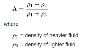
When studying hydrodynamic instabilities in density stratified flows, fluid dynamics researchers utilise the Atwood number (A), a dimensionless quantity. Mathematically:

GEOMETRY:

The geometry consists of 2 square surfaces of 20mm sides sharing one edge:

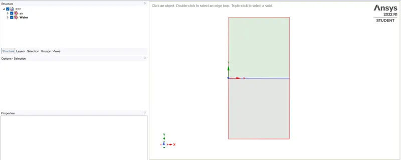
For surface prep, we have enabled the shared topology.

MESHING:

We will simulate three cases on 2 meshes. Our Baseline Mesh has an element size of 0.5mm: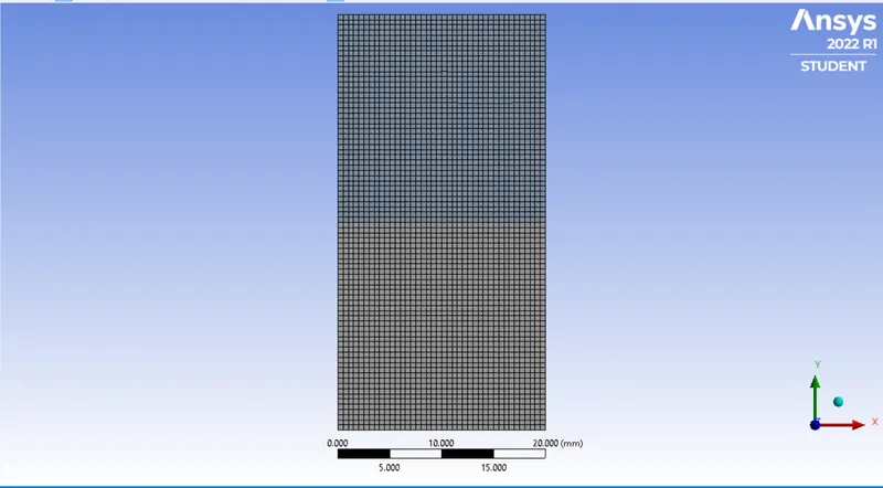

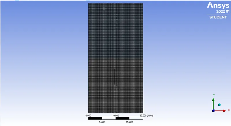
The refined mesh has an element size of 0.2mm:

SETUP:

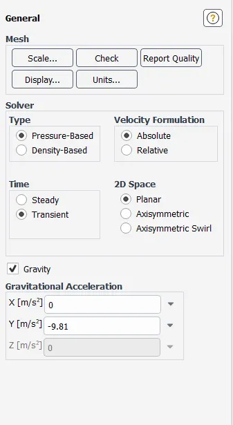
We are simulating two fluids mixing due to gravity therefore we will go ahead with the Laminar Solver. We will be using Pressure based Transient Solver with Gravity along -y:

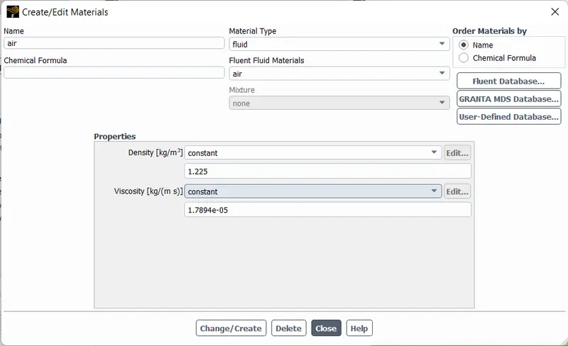
For our first two cases the fluids in question will be air:

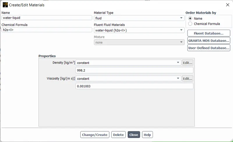
and Water:

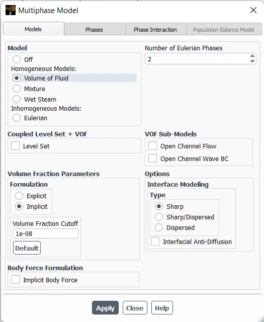
We have to also enable the Multiphase Solver:

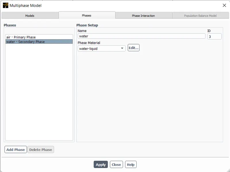
Once we are done with this basic setup, we have to initialize our case and Patch the appropriate volume fraction of the fluid:

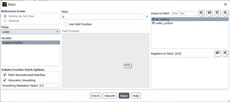
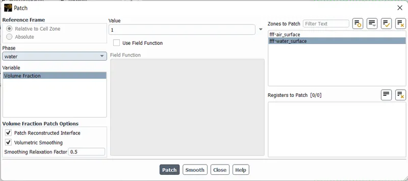
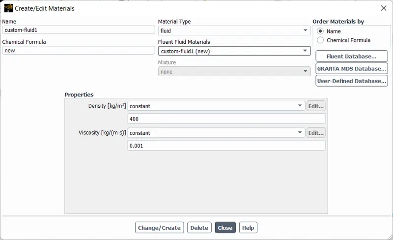
For the third case we will use a custom fluid with following properties:

RESULT:

CASE 1:

Mesh Size: 0.5 mm

Atwood Number: 0.998

Fluids: Air and Water

An animation for the simulation has been included below:

Baseline Animation

CASE 2:

Mesh Size: 0.2 mm

Atwood Number: 0.998

Fluids: Air and Water

An animation for the simulation has been included below:

Refined Animation

CASE 3:

Mesh Size: 0.2 mm

Atwood Number: 0.4

Fluids: Air and Custom-Fluid

An animation for the simulation has been included below:

Water-Custom Fluid Animation

CONCLUSIONS:

For Atwood Number:

• The simulations show that when water is injected into the air and produces enormous bubbles, air expands and produces larger bubbles. The Atwood number is estimated to be 0.998 in the first two cases and 0.4in the third case.
• The bubble and mushroom head shapes are generally symmetrical for low Atwood numbers, and the disturbances are linear.
• However, for big Atwood numbers, the shape of the bubble and the mushroom head is asymmetrical and happens fast, causing a nonlinear growth rate, at an escalating rate.
• Atwood Number closer to 0 creates symmetric finger-like figures of fluid, but if it's close to 1 then bigger bubble-like plumes develop from the much lighter fluid.

Preference for Transient Solver:

We prefer the transient solver so that we can see the real-time changes in the simulation. A steady-state solution is focused on getting the end result, in RT Instability we are more observant of the bubble and vortex formation hence, the process is more important than the end result.

Mesh Inferences:

A finer mesh reveals the vortex formation and bubbles in a more resolved and clear way, compared to a coarse mesh. The vortex and bubbles can be explicitly seen in case 2 and 3 whereas in case 1 they are comparatively more ambiguous.