Week 5 - Rayleigh Taylor Instability
Aim
To demostrate a Rayleigh-taylor instability
Objectives
Some practical models based on Rayleigh-Taylor waves
1.Saffman-Taylor instability
Also called as viscous fingering it occurs when a less viscous fluid is injected displacing a more viscous fluid.In a CFD application this method is usually observed in Hele-Shaw cells which consist of two closely spaced, parallel sheets of glass containing a viscous fluid. The two most common set-ups are the channel configuration, in which the less viscous fluid is injected at one end of the channel, and the radial configuration, in which the less viscous fluid is injected at the centre of the cell. Instabilities analogous to viscous fingering can also be self-generated in biological systems.
2.Richtmyer-Meshkov instability
This occurs when 2 fluids of different density are impulsively accelerated.The multiphase Richtmyer–Meshkov instability (RMI) often occurs in supernova events and inertial confinement fusion processes, where it plays a critical role. In the evolution of the RMI process, the particle phase may have either a dilute or a dense pattern.
3.Kelvin-Helmholtz instability
Kelvin-Helmholtz instability appears in stratified two-fluid flow at surface. When the relative velocity is higher than the critical relative velocity, the growth of waves occurs. The experiment of Thorpe used as a benchmark in the present paper, is made in a rectangular glass tube filled with two immiscible fluids of various densities. They simulated the growth of instability with CFX-5.7 code and compared simulation with analytical solution. It was found that surface tension force, which stabilizes growth of waves, actually has a destabilizing effect in simulation, unless very small timestep and residual is used. In CFX code system of nonlinear Navier-Stokes equations is linearised and solved iterative in each timestep, until prescribed residual is achieved. On the other hand, simulation without surface tension force is more stable than analytical result predicts.
4.Plataeu-Rayleigh instability
This explains why and how a falling stream of fluid breaks up into smaller packets with the same volume but less surface area.The well-known phenomena of Plateau–Rayleigh instability has been simulated using computational fluid dynamics (CFD). The breakup of a liquid film into an array of droplets on a cylindrical element was simulated using a volume-of-fluid (VOF) solver and compared to experimental observations and existing theory. It is demonstrated that the VOF method can correctly predict the breakup of thins films into an array of either axisymmetric droplets or clam-shell droplets, depending on the surface energy. The existence of unrealistically large films is precluded. Droplet spacing was found to show reasonable agreement with theory. Droplet motion and displacement under fluid flow was also examined and compared to that in previous studies. It was found that the presence of air flow around the droplet does not influence the stable film thickness; however, it reduces the time required for droplet formation. Novel relationships for droplet displacement were derived from the results.
Results
Case 1
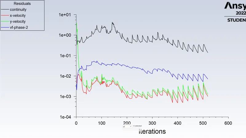
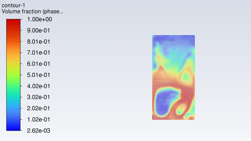
Mesh = 0.5mm
Case 2
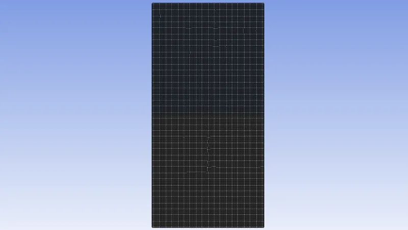
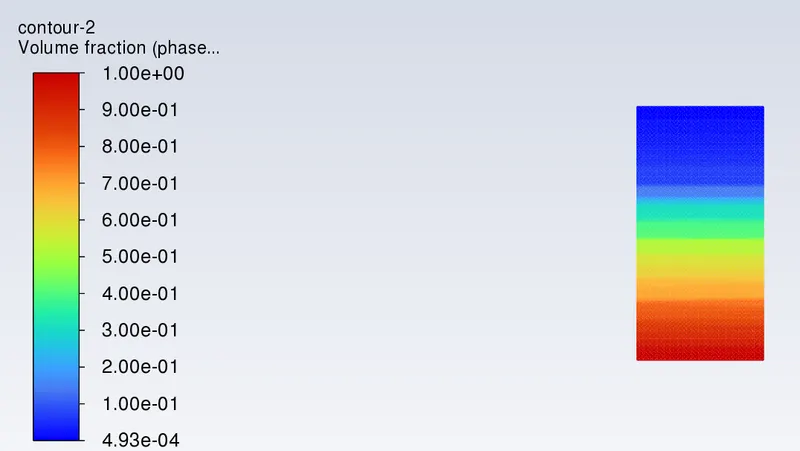
Mesh size = 0.2mm
Cells = 200000
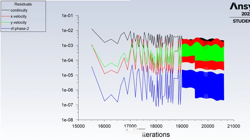
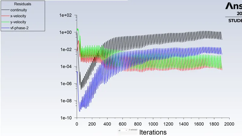
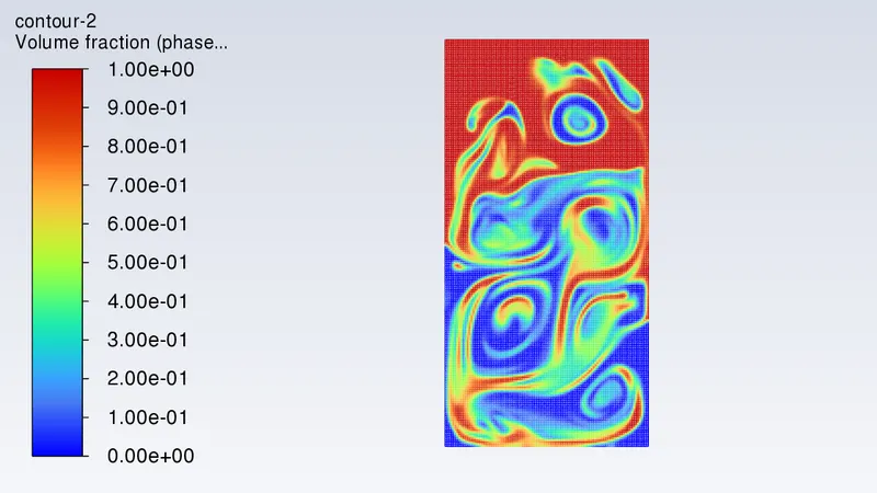
Case 3
In this case the mesh size remians the same only the values are changed . Here,instead of air a user defined material of density 400kg/m^3 & viscosity of 0.001 kg/m-s is used.
Atwood number
It is a dimensionless number in fluid dynamics used in the study of hydrodynamic instabilities in density stratified flows.
`A=(rho1-rho2)/(rho1+rho2`)
ρ">ρ1 --> Density of heavier fluid
ρ">ρ2 --> Density of lighter fluid
Case 1
Density of air = 1.225 kg/m^3
Density of water = 998.2 kg/m^3
A = `(998.2-1.225)/(998.2+1.225)`= 0.997
Case 2 will be same as only the mesh is different
Case 3
Density of water = 998.2 kg/m^3
Density of User defined fluid = 400 kg/m^3
A = `(998.2-400)/(998.2+400)`= 0.427
From the above Atwood values we can say that as the density of the lighter fluid increases the Atwood number is decreasing due to this the disturbances and permutations are linear for a larger time.For a larger Atwood number the disturbances occurs very rapidly at a accelerating rate which leads to non linear growth rate.