Week 5 - Rayleigh Taylor Instability
*** RAYLEIGH TAYLOR INSTABILITY ***
::::::::::::::::::::::::::::::::::::::::::::::::::::::::::::::::::::::::::::::::::::::::::::::::::::::::::::::::::::::::::::::::::::::::::::::::::::::::::::::::::::::::::::::::::::::::::::::::::::::::::::::::::::::::::::::::::::::::::::::::::::::::::::::::::::::::::::::::::::::::::::::::::::::
- AIM - Modelling mixing of two fluids having different densities to observe the Rayleigh Taylor instability at the interface. To address different concepts related to the models used in RTI, Atwood number, and Courant number.
- INTRODUCTION -
The Rayleigh Taylor instability or RT instability (after Lord Rayleigh and G. I. Taylor) is the instability of an interface between two fluids of different densities which occurs when lighter fluid pushes the heavier fluid. It is a dynamic process where two fluids seek to reduce their combined potential difference. When the higher density fluid tries to mix with the fluid having a lighter density, the gravity acts downward. Then lighter tries to rise in the response to the downward motion of the heavier fluid. This creates a basic platform for the Rayleigh-Taylor instability, in further study motion, shape direction, reaction and behavior observed and analyzed. In Rayleigh-Taylor instability, viscosity does play an important role it slows down the instability to observe it properly. High viscosity reduces Reynold's number hence prevents turbulence hence the shape observed pretty well. The mixing of fluid with different density rates over one another is called density stratification.
The Rayleigh-Taylor is a fingering instability of an interface between two fluids of different densities. The various example of Rayleigh-Taylor Instability explains the behavior of the overturn of the collapsed core of a massive star, for the motion of high luminosity jets in rotating gas clouds in the external gravitational potential, the electromagnetic implosion of the metal liner, the explosion of atomic bomb and supernovas, etc.
- THEORY -
- Multiphysics Modeling -
Multiphysics involves the analysis of multiple simultaneous physical phenomena. This simultaneous phenomenon can include heat transfer, fluid flow, deformation, electromagnetics, acoustics, and mass transport. Despite the complexity involves in coupling multiphysics is essential for many applications where traditional single physics analysis is inadequate. Multiphase flows can be numerically calculated using the Euler-Lagrange approach or the Euler-Euler approach. The volume of fluid (VOF) is a type of Euler-Euler approach, it is basically a surface tracking technique. Usually used if there are more than two immersible fluids, where interface position is of importance. it has only one set of momentum equations, shared by all fluids and volume fractions of each of the entire system. Very useful to simulate interface resolved physical problems such as droplet and bubble hydrodynamics, heat and mass transfer phenomenon in drops and bubble can also be simulated. VOF model will be more useful if the study is focused on interface tracking.
In computational fluid dynamics, the volume of fluid (VOF) is a free surface modeling technique, i.e. a numerical technique for tracking and locating the free surface (or fluid-fluid interface). It belongs to the class of the eulerian method which is characterized by mesh that is either moving or stationary in a certain prescribed manner. As such volume of fluid (VOF) is an advection scheme a numerical method allows to track shape and position of the interface, but it is not a standalone flow solving algorithm. It is a scalar function, defines the integral of the characteristics of the fluid function in a control volume when the cell is empty the value of C is zero and when C=1 the cell is full, and when there is a fluid interface in the cell is a discontinuous function.
The various multiphysics models are Algebraic Interfacial Area Density (AIAD), Eulerian Model, Mixture Model, Population Balance Model, Discrete Phase Model (DPM), VOF to DPM Model, Dense Discrete Phase Model, Discrete Element Method. Based on the problem the different models are used, in our case, we are stick with the volume of fluid (VOF) model.
- COURANT NUMBER (CFL NUMBER)-
In mathematics, the Courant-Friedrichs-Lewy condition is necessary to condition for convergence while solving certain partial differential equations numerically by the method of finite differences. It arises in the numerical analysis of explicit time-marching schemes when these are used for the numerical solution. As a consequence, the time step must be less than a certain time in many explicit time-marching computer simulations, otherwise, the simulation will produce an incorrect result. The condition is named after Richard Courant, Kurt Friedrichs, and Hans Lewy who described in 1928.
In 1D cells, to identify the courant number let's consider a rectangular cell. In that flow field, the fluid flows from left to right represented by U profile, and `Delta x` represents the total length of the cell as shown in the figure. Over the time step delta T, the velocity approaches in the cell with the distance of Udeltat of the cell having the length of delta x across the cell. The bigger is the time step `Deltat` further the distance covered by `U Delta t`. Now the courant number defines as the ratio of the distance flow covered (`U Delta t`) to the length of the cell (`Delta x`) or The fraction of the cell that the flow moves across in the time step.
`Co = (Fluid Distance)/(Cell Distance) = (U Delta t)/(Delta x)`
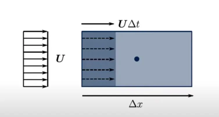
Fig No. 1. 1D cell representation in a rectangular format to compare the length scale.
If Co = 0.3 then the flow distance covers 30% of the length of the cell and if Co = 1.1 then the flow of fluid covers or surpasses the length of the cell in a single timestep.
In 3D, the system courant number behaves differently keeping the basic definition the same because of the irregular shape of the 3D cell or skewness in element quality. If the cells are not in perfect shape then the system of calculating courant number needs to modify accordingly for this purpose need to define the length of flow in a particular cell in the particular cell according to the orientation of the cell. The distance across the cell can be defined as -
`Delta x = (Cell Volume)/ (Total Surface Area) = V/A`
Total surface area can be defined as the sum of the surface area/ length of the face of the cell.
A = A1 + A2 + A3 + ........... + An.
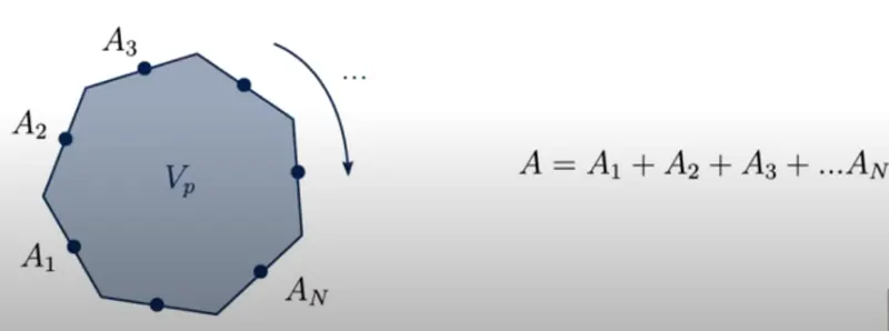
Fig No.2. 3D cells surface area calculation and the orientation calculation complexity.
Now for the velocity, have to find the velocity normal to the face. Also need to understand the condition of conservation of mass. This creates a problem of the sum of velocity normal results in zero. To avoid this needs to take magnitude and divide with 1/2 to get the actual velocity flux normal to face. The final definition of courant number for an arbitrary shaped 3D cell can be represented as,
Velocity flux = `sum(1/2*U_f*n_f)`
`Co = 1/2*Deltat * ((sum|U_f*n_f)/V_p)`
The courant number should be considered as a field because every cell in the mesh has a different courant number. Hence, it is a field and can be plotted like any other variable such as temperature, velocity, and pressure. Most often the maximum courant number should be below 1.0.
- TIMESTEPPING SCHEME -
Fixed time-stepping - Choose a time step size `Delta t` then CFD solver computes the flow field U and compute Co courant number for every cell. Then proceed to the next iteration keeping `Delta t` the same also `Delta x` will remain fixed over a simulation. The CFD solver continues the procedure, if the courant number is too large the solution may diverge or Crashdown. Now have to go back to change manually the timestep and rerun the simulation.
Adjustable time-stepping - In such scenarios, to avoid the complexity of time stepping better option is to use an automatic adjustable time-stepping scheme rather than a fixed time step. In the adjustable time-stepping scheme, initial time step size `Deltat` and maximum courant number Comax are provided. CFD solver computes flow field U then finds Co. If Co > Comax then reduces the time step `Delta t` for the next iteration. The reduction in time step `Delta t` carried out by the simple way,
`Delta t_(n) = Delta t_(old) * (Co_(max))/(Co)`
But it creates the problem of very rapidly changing the time step which creates oscillation and it may diverge the solution or disturb the accuracy. Now in such case have to use either relaxation or limiting to prevent large change in `Delta t`.
- Practical CFD models that have been based on the mathematical analysis of Rayleigh-Taylor waves and explain how these mathematical models have been adopted for CFD calculations -
- 1D Rayleigh-Taylor Mixing -
The turbulence models have been applied to the simulation of simple 1D Rayleigh-Taylor mixing cases with a 3:1 density ratio. The computational domain extends with heavy fluid placed on the left side of the domain and initial interface at x=0. Unless otherwise stated, the computational grid consists of 100 cells and the adiabatic exponent is `gamma = 5/3` for both fluids. The following relation satisfied in all cases when Aog = 1; thus for the 3:1 density ratio the gravitational acceleration is g = 2 cm/s^2.
- Tilted-RIG Rayleigh-Taylor Mixing -
The tilted-RIG test case originates from a series of experiments performed to study the mixing between two variable densities of fluid induced by Rayleigh-Taylor instability. In the experiment tank containing two fluids of different densities, heavy fluid places below the lighter fluid in the tank is accelerated downwards between two parallel guide rods using firing rocket motors. The downward acceleration caused the to tank effectively changes the direction of gravity (external body force) so that system becomes Rayleigh-Taylor unstable, causing the two fluids to mix. The acceleration from the rocket was not constant but approximately averaged as 35 times normal gravity. It eventually attains roughly constant value but the time during which acceleration varies is significant and still needs to consider one approach is to directly incorporate measured value into the simulation (i.e. variable gravity g(t)). This works well for incompressible Navier-Stocks solver; however, it can create problems for compressible codes. An alternative approach is to make use of constant acceleration for which a non-dimensional time T is used for comparison with experimental results.
`tau = intsqrt((A_t*g_z)/L_x)*dt + delta`
- SPRAY BREAKUP MODELING -
a. CHU Breakup model -
The Rayleigh-Taylor instability form the basis of model formulated by Chu. The theoretical correlation constructed in order to predict droplet size based on experimental function which was used in fuel-coolant interaction models. The model implemented in this study represents the modified version of the Chu's original model in that it includes a Taylor-series expansion of the exponential term to first order and subsequently on explicit discretization in time in which drop diameter correlation is written as :
`dD/dt = - Co* C1 * W_e^(C2)*(u_(rel)*epsilon^0.5) * tau^ast(C1-1)`
`Co = 0.1708 - 0.149 * epsilon^0.5`
`epsilon = rho_g/rho_1`
`tau^ast = (epsilon^0.5* u_(rel)^t)/D_o`
`C1 = 0.772 , and C2 = 0.246`
b. Wave Model -
The wave model (KH Model) was proposed by Reitz. The model is based on a first-order linear analysis of Kelvin-Helmholtz instability growing on the surface of the cylindrical liquid jet with an initial diameter that is penetrating the stationary incompressible gas with relative velocity Urel as shown in the figure.
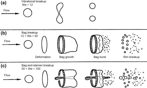
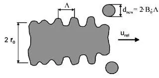
Fig No.3. Wave model illustration.
The instability at the surface is small axisymmetric displacement (`eta`).
`eta = eta_0*e^(ikz + wt)`
where `eta_0` is an infinitesimal initial perturbation, k is wave number, w is the growth rate.
Wavelength `lambda`is related to the wavenumber as `lambda = (2 pi)/k`.
c. KHRT Model -
It is known that liquid droplets in diesel sprays have very high initial velocities and decelerate rapidly due to drag forces. In this case, Rayleigh-Taylor instability may also plays important role in the droplet breakup mechanism in addition to Kelvin-Helmholtz instability as shown in the figure.
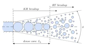
Fig No. 4. Kelvin-Helmholtz and Rayleigh-Taylor targeted spectrum while modeling.
In the KHRT model, the aerodynamic force on the drop flattens it into the shape of a liquid sheet and the decelerating sheets break into large-scale fragments by means of Rayleigh-Taylor instability. KH waves with a much shorter wavelength originate at the edge of the fragments and these waves break into micrometer-sized droplets as illustrated in the figure.
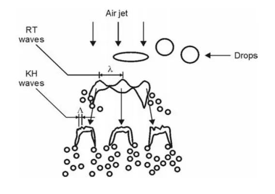
Fig No. 5. KHRT waves comparison.
- MASS DIFFUSION MODEL -
The mass diffusion equation describes the transport of mass and energy due to model viscosity and hence drives the mixing in the fluids. Even if any configuration is Rayleigh-Taylor unstable, diffusion processes could responsible for significant mixing in the viscosity is significantly large.
- SINGLE FLUID MODEL -
a. Potential Flow Model -
The potential flow model first used by Layzer (1955) this model valid for instability stages from the linear stage through the early non-linear stages to the asymptotic but limited to A = 1. In this model, single-mode perturbation and expand the flow equations to the second-order around the bubble tips, hence obtaining an ordinary differential equation for the bubble velocity.
b. Buoyancy Drag Model -
Buoyancy-drag models valid for every Atwood number but limited to the non-linear stages of instability. It uses an ordinary differential equation to evolve the width of the mixing layer. The bubble or spikes, the amplitude is described by the balancing inertia; buoyancy, and drag forces. These models cannot model multiple mixing interfaces; cannot be easily extended to two or three dimensions and as the rule do not address the demixing also known as counter gradient transport i.e. reduction of total fluid masses within the mixing zone. To address the above problem two-fluid or multi-fluid models are used.
c. Besnard-Harlow-Rauenzahn Model (BHR) -
It is a more advanced version of the single-fluid model. The BHR model based on the evolution equation arising from second-order correlation and gradient-diffusion approximations. Using mass-weighted average decomposition, the original BHR model includes a full transport equation for the Reynold stresses, turbulent mass-flux velocity, density fluctuation, and the turbulence kinetic energy dissipation rate.
- MULTI-FLUID MODEL (TURBULENCE MIXING MODEL) -
The multi-fluid model uses a separate set of the equation to each fluid in addition o the main flow equation and provide an accurate modeling framework for demixing by correctly capturing the relative motion of the different fluid fragments.
a. Two equation K-L Turbulence model -
The K-L turbulence equation evolves the equation for turbulence kinetic energy (K) and turbulence length scale (L). The model was developed by Dimonte and Tiptone for describing the turbulent self-similar regime of Rayleigh-Taylor instability-induced mixing. The starting point deriving the model equation is buoyancy-drag model s for self-similar growth of Rayleigh-Taylor instability.
b. Three equation K-L-a Turbulence Model -
The three equation of Morgan and Wickett was developed as an extension to the two-equation K-L model of Dimonte and Tiptone by including third equation for turbulent mass-flux velocity.
c. Four equation K-L-a-b Turbulence Model -
It is an extension to the K-L-a model by adding an evolution equation for the density-specific volume covariance. This model can accurately reflect the effects of the changes in density fluctuations.
- CFD ANALYSIS OF RAYLEIGH-TAYLOR INSTABILITY -
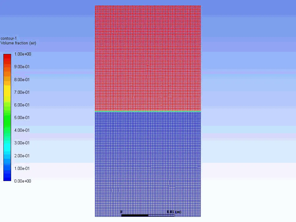
The analysis is done for three different cases by increasing the number of cells. As its multi-fluid analysis, VOF method influent is used and implicit solver with active implicit body force chosen. Choosing the accurate time step is more important to capture the instabilities at the interface as well as in the fluid zones. The idea is that the dense fluid water is at the top and light fluid air is at the bottom and due to gravity, there will be instability at their interface, which is going to be calculated by using VOF multiphase method in ANSYS.
The equilibrium here is unstable to any perturbation or the disturbances at the interfaces the potential energy of the configuration is lower than the initial state, thus the disturbances will grow and further release the potential energy as the more dense material moves down under the effective gravitational field and the less dense material is further displayed upwards. This was set up as studied by Lord Rayleigh.
- GEOMETRY DETAILS -
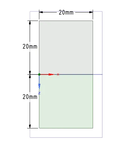
Fig No.6. Geometry details
1. BASELINE MESH AND ITS MESH METRICS AT 0.5MM BASE MESH -
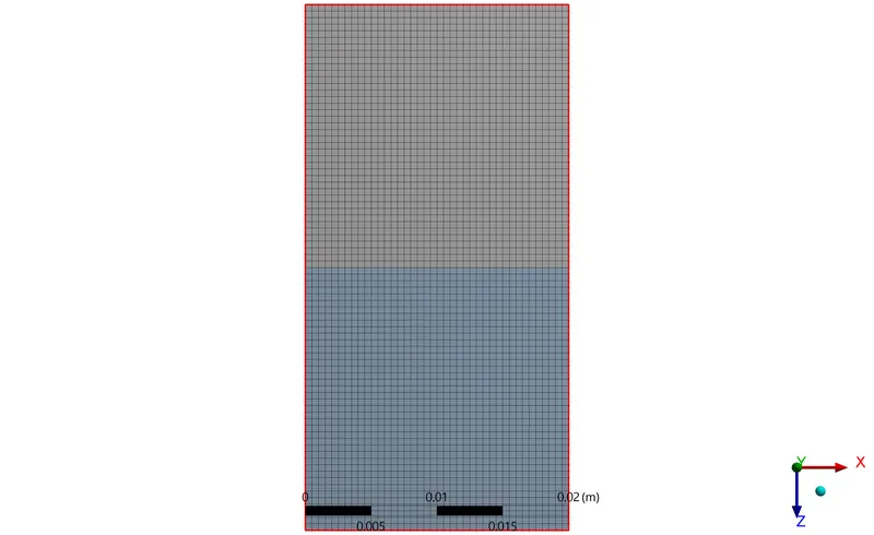
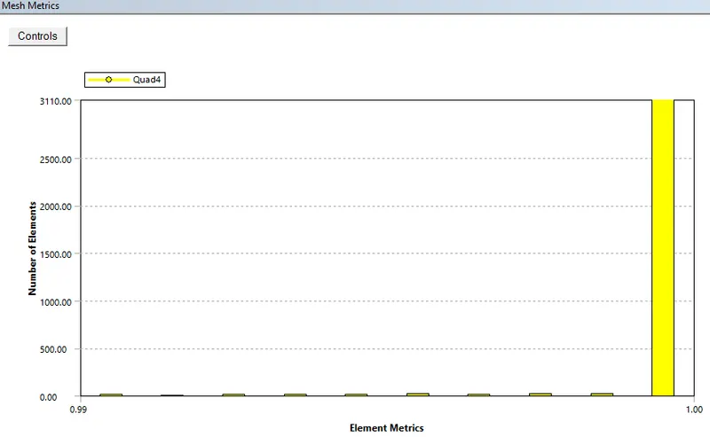
Fig No.7. Mesh and its mesh metrics at 0.5 mm base mesh.
2. REFINED MESH AND ITS MESH METRICS AT 0.2 MM MESH SIZE -
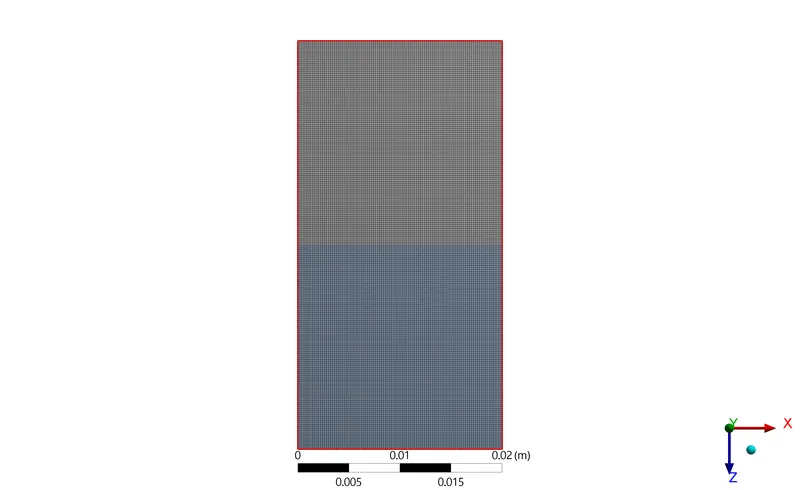
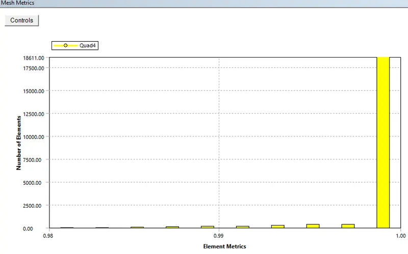
Fig No.8. Mesh and its mesh metrics at 0.2 mm base mesh.
- SETUP -
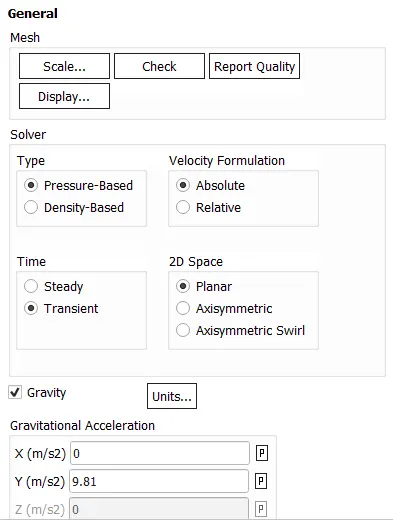
Fig No.9. General Setup and gravitational acceleration.
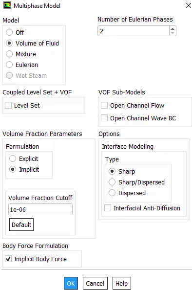
Fig No.10. Multiphase model.
In the multiphase model, the implicit method for the formulation is used by keeping on the body force formulation.
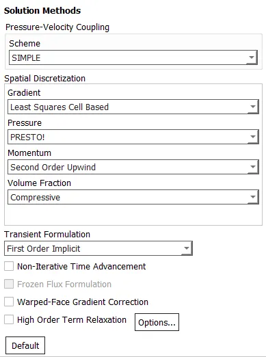
Fig No.11. Solution Methods.
- RESULTS -
1. The RTI analysis under the gravitational acceleration of the 9.81m/s^2 at 0.5 mm base mesh by providing default material of air and water.
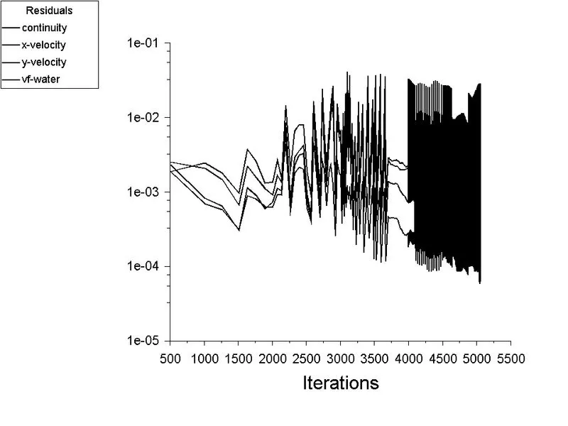
Fig No. 11. Residual.
2. The RTI analysis under the gravitational acceleration of the 9.81m/s^2 at 0.2 mm base mesh by providing default material of air and water.
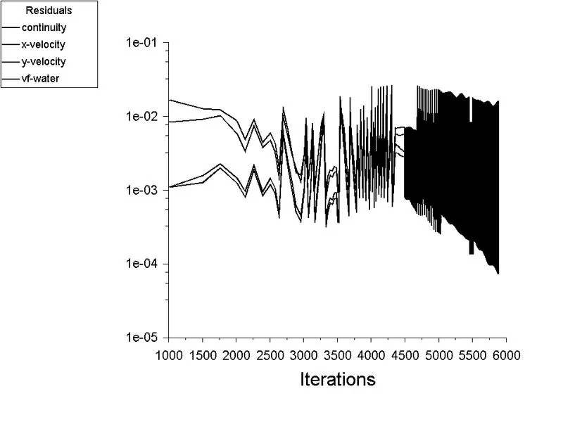
Fig No. 12. Residual.
3. The RTI analysis under the gravitational acceleration of 9.81 m/s^2 at 0.2 mm mesh size and the heavier fluid is the default water provided by the Ansys and lighter user-defined fluid used having the density of 400 Kg/m^3 and the viscosity of 0.001 Kg/m-s.
RTI analysis carried out under the gravitational acceleration under this case to observe the turbulence created by the instability in a better manner instead of the air the user-defined lighter fluid is used with density to be 400 kg/m^3 and viscosity is 0.001 kg/m-s.
- OBSERVATIONS -
In the above cases, the simulation starts with the state of hydrostatic equilibrium, and Rayleigh-Taylor is observed when a lower density fluid pushes the higher density fluid due to which formation of shock waves at the interference takes place and formation of the bubbles take place, which compresses the heavy fluid around it, due to which shock waves of multidimensional fashion generates and it gets stronger as it moves upwards.
It is observed that the more we refine the mesh the simulations results get smoother about the irregularities that take palace at the interference of two fluids. As higher density fluid replaces lower density fluid, the formation of air bubbles takes place which travels towards the upward region with time. In the third case, we can see the more detailed result about the information of waves and formation of an air bubble that gets trapped at the lower region during the initial stage and then they travel toward the upper region, generating shock waves. At the end of the simulations it is to be observed that the two phases get separated from each other though, we can see some diffusivity between them which is a volume fraction of air and water.
- Why steady-state approach might not be suitable for the above type of simulations?
The differences between the steady and transient are that you cant see the small-time variation of instability. The steady-state simulation is performed if we are concerned to learn about the transition of the irregularities that starts developing when we pour high dense fluid upon low dense fluid under gravity effects so, by using the transient solver along with refined mesh of the model, we can compute the smooth transition of irregularities that takes place at the interface of the fluids. The final state results for both the steady-state and transient state will be the same.
- ATWOOD NUMBER -
The Atwood number (A) is a dimensionless number in fluid dynamics used in the study of hydrodynamics instabilities in density stratified flows. It is a dimensionless density ratio as defined as :
For the first case :
`A = (rho_1 - rho_2)/(rho_1 + rho_2) = (998.2-1.25)/(998.2+1.25) = 0.99749`
For the second case :
`A = (rho_1 - rho_2)/(rho_1 + rho_2) = (998.2-400)/(998.2+400) = 0.4278`
Rayleigh-Taylor instability evolves in three different stages namely linear stability, mushroom head formation, and long-term evolution. For Atwood numbers close to zero Rayleigh-Taylor instability flow takes the form of asymmetric spikes of the fluid; For Atwood numbers close to 1 the much lighter fluid below the heavier fluid takes the form of larger bubble-like plumes. This process occurs very rapidly thus suggests that it may be the result of a transition to turbulence in the flow. A larger Atwood number leads to larger acceleration and which makes the growth rate non-linear.
The calculated Atwood number is close to 1 and from the simulation results, it is found that when high dense fluid i.e. water poured upon low dense fluid i.e. air under gravity, the formation of air bubble-like plumes takes place which travels towards the upward region in the form of waves and some gets trapped at the lower region during the initial stages, which afterward try to move toward the upper region and at the end, both phases get separated with some diffusivity left at the middle portion between them. Thus the calculated Atwood number is validated for our simulation results.
- CONCLUSION -
- Choosing the wrong timestep leads to floating-point error.
- The way to smaller timesteps will not provide the solution at all. To avoid such a problem adjustable time step should use.
- Instabilities are captured when the mesh size is smaller but, it certainly needs more time for calculations.
- The third case shows larger turbulence generated and vortices form.
- In all simulation results, when the fluid gets to settle down one can observe that the mixing and diffusion of the fluid at the center of the geometry.
- It is quite difficult to understand in the first two cases when the air and water are used as the fluid when the solution gets to settle down one can observe the mixing of phases in the center or the reduction in the number of fluids which cannot happen at normal circumstances.
- References -
2. https://permalink.lanl.gov/object/tr?what=info:lanl-repo/lareport/LA-UR-83-2130