Week 3 - External flow simulation over an Ahmed body.

`***`AHMED BODY CHALLENGE`***`

• AIM - External aerodynamics flow simulation over Ahmed body solved by using steady-state to identify the reason for negative wake region and to perform grid independency test.

• INTRODUCTION -

The flow around road vehicles (car, buses, truck) under normal operating conditions is principally turbulent. It is typically characterized by large scale separation and recirculating regions, a complex wake flows long trailing vortices, and interaction of boundary layer flow on vehicle and ground. In the design of ground vehicles, the crucial part is to decide the turbulent model according to the type of vehicle. The advanced modeling techniques and solving methods require hours and days of work for CPUs to calculate at precision. In aerodynamic flow around a vehicle, it is a three-dimensional flow and the design will have an influence on principle features such as the shape of the vehicle, aerodynamic drag, fuel consumption, noise production, and road handling.

By using wind tunnel experiments the designer have an understanding of airflow around the vehicle through extensive wind tunnel testing. But wind tunnel testing for every prototype is a time-consuming and costly process. Also, the reliability of the turbulence model and its long-lasting process of calculation is another challenge. In order to reduce time, it is necessary to use simplified computational technic and adopt a model to describe the mean effect of turbulence. Unfortunately, a simple turbulence model often fails to calculate the flow properly especially the position of flow separation on the rear slant is crucial in determining the aerodynamic drag but is an extremely difficult feature to calculate. To overcome the problem, S. R. Ahmed in 1984 described an Ahmed body with the standard results to test the various type of challenges and turbulence models. Ahmed body is a kind of baseline bluff body geometry for automobile bodies.

People working in vehicle aerodynamics use Ahmed body to validate their numerical model because experimental data from wind tunnel testing is available for Ahmed body. Once the numerical model is validated it is used to design new models of the ground vehicles.

• THEORY -

The geometry of the vehicle is complex, the flow around the vehicle is fully three-dimensional, boundary layers are turbulent flow separation and there are large turbulent wakes in which longitudinal trailing vortices are common. Typically for the bluff body, the principal contribution to drag experienced by road vehicles is pressure drag, and an important objective of vehicle aerodynamic design is the avoidance, reduction, or control separation. Viscous-inviscid flow interaction can be challenging to predict for any bluff body separated flow and this is particularly so when there are ground effects present,

A bluff body is a body that as a result of its shape has separated flow over a substantial part of its surface. The bluff body has a very strong interaction between viscous and inviscid regions. Consider that at the moment of starting the flow is attached. Prediction of separation position from a continuous surface is particularly difficult because it depends on both the characteristics of the upstream boundary layer and on the structure of the near wake region. Usually, bodies induce a separation region where velocity at the edge of the boundary layer is higher than free stream velocity.

In this technical report, a) we will be conducting an external aerodynamic flow on Ahmed body by placing it in the enclosure to the motion of air over it at 25 m/s. This will be done to analyze drag, lift, vector plots near the wake region and pressure experienced by the body.

b) Also motive to find the reason of negative pressure in wake region and the explanation on the significance of point of separation.

c) The grid independency test is carried out to get the correct result possible for every iteration of the problem.

• BOUNDARY LAYER -

The boundary layer is a thin layer of a real fluid along the surface of an object in which viscosity effects fluid dynamics. When fluid flows over a plate, velocity near the surface much lower, and vorticity is present. The no-slip condition accounts for zero relative velocity at the plate and keeps on increasing until it reaches the free stream velocity U`oo`. The fluid deceleration is transferred from one fluid layer to another fluid layer by viscosity and it forms a velocity gradient in the boundary layer.

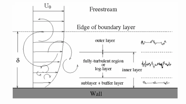
Fig No. 1. Boundary layer thickness. Source: Ansys Documentation.

Since we dealing with the turbulent boundary layer and related phenomenon from the above figure it can be seen that in the turbulent boundary layer region flow near the wall has been analyzed in terms of three layers.

1. The inner layer or sublayer where viscous shear dominates.
2. The outer layer or defect layer, where large scale turbulent eddy shear dominates.
3. The overlapping layer or log layer where velocity profiles exhibit a logarithmic variation.

Near to the wall the flow is influenced by the viscous effects and independent of free stream parameters. However, the mean flow velocity depends on the distance from the wall(y), fluid density(`rho`), viscosity(`mu`), and wall shear stress(`tau`).

• Y+ :

Turbulent flows over a body is an essential phenomenon in computational fluid dynamics and are significantly affected by the shape of the body where viscosity affected regions have larger gradients in the solution variable. An accurate representation of the near-wall region determines a successful prediction of wall-bounded turbulent flows.

The reason for the need for Y+ is to distinguish different regions near the wall or in the viscous region. If we intend to resolve the effects near the well that is in the viscous sublayer then the size of the mesh should be small and dense enough near the wall so that almost all the effects are captured. The smallness, in this case, varies from problem to problem to identify the size Y+ comes into play. Based on the Y+ value first cell height can be calculated. The near-wall region is meshed using the calculated first cell height value with gradual growth in the mesh size so that the effects are captured and avoiding overall heavy mesh count.

Below the law of wall is finally displayed clearly and we can see four different length scales:

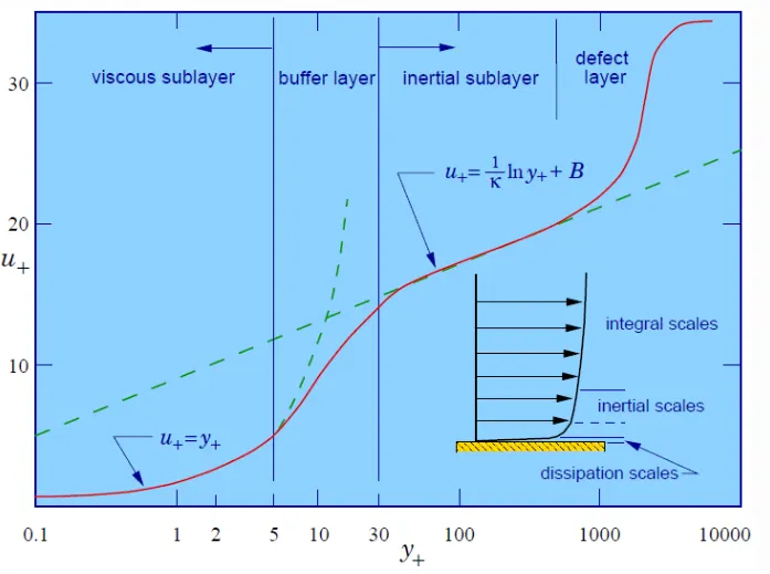
Fig No. 2. Y+ VS U+. Source: Skill Lync.

The above plot is a log-log plot, which means the curved line is linear variation and a straight line is a logarithmic variation. The existence of all these layers in the boundary layers made the near-wall treatment nonlinear and inconsistent. In 1905, Prandtl and his student Nikuradse normalized the axes into Y+ (The axis that is used to be the distance) and U+ (The axis that is used to be the velocity). They also wrote an equation that would fit U+ and Y+ near the wall. In the terms of Y+ value, we can say that

1. In viscous sublayer - 1 < Y+ < 5
2. In the transition layer - 5 < Y+ < 30
3. In the log layer - 30 < Y+ < 500

From the above discussion, we can say that placing the first cell in the mesh region is very vital to determine the turbulent model as well as to compensate on the computational mesh and the time Y+ value for our case is in viscous sublayer so that we choose it is to be Y+ = 1.

Calculation of Y+ :

1. Determine the skin friction coefficient -

`Cf = 0.0576*(Re)^(-1/5)`

2. Wall shear stress `tau_w` can be calculated from skin friction coefficient, `Cf`

`tau_w = 1/2*Cf*rho*U_oo^2`

3. Calculate `U_T`

`U_t = sqrt(tau_w/rho)`

4. Now write the definition of Y+ and rearrange it for Y+

`Y+ = ((y*U_T)/nu) -> y = ((Y+*nu)/U_T)`

In our case, Y+ value calculated as follows:

1. Reynold number - From the default material provided for air. `rho = 1.225 ((kg)/m^3) and mu = 1.7894e-5 ((kg-m)/s)`

`Re = ((rho*u*D)/mu) = ((1.225*1.044.25)/(1.7894e^-5)) = 1786772.102` This belongs to turbulent nature of fluid.

2. Skin friction coefficient for turbulent flow -

`Cf = 0.0576*(Re)^(-1/5) = 3.236 * 10^-3`

3. Wall shear stress, `tau_w`

`tau_w = 1/2*Cf*rho*U_oo^2 = 1.23878`

4. Calculate `U_T`

`U_T = sqrt(tau_w/rho) = 1.0056`

5. calculate for y and we are using Y+ = 1 for viscous sublayer,

`y = ((Y+*nu)/U_T) = ((1*1.7894*10^-5)/(1.225*1.0056)) = 1.426*10^-5 m`

The first layer thickness for the external flow over Ahmed body calculation and simulation is 1.426*10^-5 m.

For making accurate predictions of near-wall, the mesh resolution modeling approach is equally important. The model of choice and grid resolution are tightly coupled in the sense that a very good model for a specific application will achieve acceptable prediction only if the mesh resolution matches the chosen specific model.

------------------------------------------------------------------------------------------------------------------------------------------

• SOLVING & MODELING APPROACH -

The analysis of external flow over Ahmed body is carried out in a steady-state because the main objective of the report is to demonstrate the simulation and produce drag & lift plots. In the first place, the basic mesh is used in the discretization of the domain to generate baseline simulation. Then step by step will improve the mesh carried out the grid independency test until results vary very slowly. The pressure & velocity contours and coefficient of drag & lift plots are generated in this analysis.

The k-epsilon, RSM, LES model are primarily valid for turbulent core flows that is region somewhat far from the wall. The Spalart-Allamaras and K-Omega models were designed to apply throughout the boundary layer.

• K-Omega model -

This model takes elliptic near-wall behavior meaning that it has an inherent nature of being able to "communicate" with the wall and actually has Dirichlet boundary conditions. The implication of such behavior is the straight forward possibility of integrating through the laminar sublayer without additional numerically normalizing damping functions or two additional transport equations. Commonly encountered situations where the flow demands integrating through the viscous sublayer includes heat transfer, aerodynamic drag, flow with an adverse pressure gradient, etc. for such application we have used the k-omega model to simulate flow over the Ahmed body.

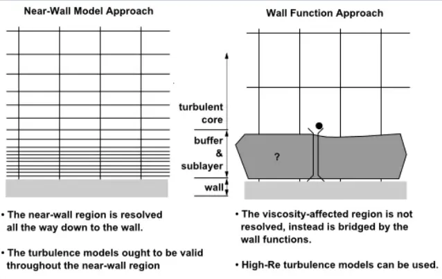
Fig No. 3. Near wall model approach. Source: Ansys Documentation

--------------------------------------------------------------------------------------------------------------------------------------------

• GEOMETRY DETAILS -

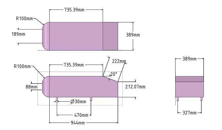
Fig No. 4. Geometry Details

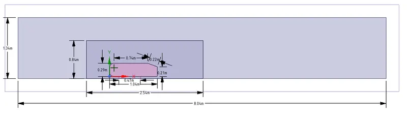
Fig No. 5. Side View with Enclosures

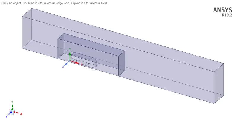
FIg No. 6. Isometric Cross-sectional view after using the split-body tool.

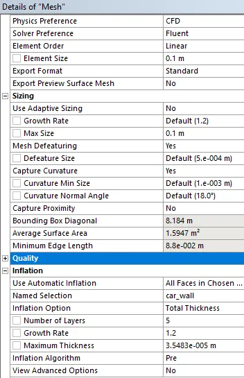
Fig no. 7. Mesh Details

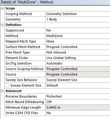
Fig No. 8. Multizone mesh details for the outer enclosure.

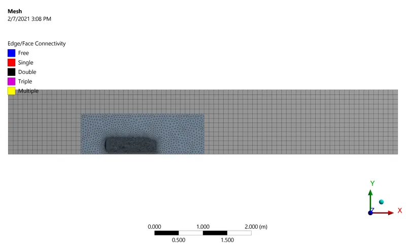
Fig No. 9. Multizone mesh on the outer enclosure.

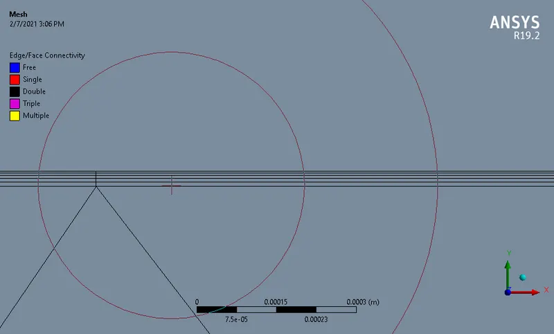
Fig No. 10. Inflation Layer on the boundary of the Ahmed Body.

---------------------------------------------------------------------------------------------------------------------------------------

• Setup -

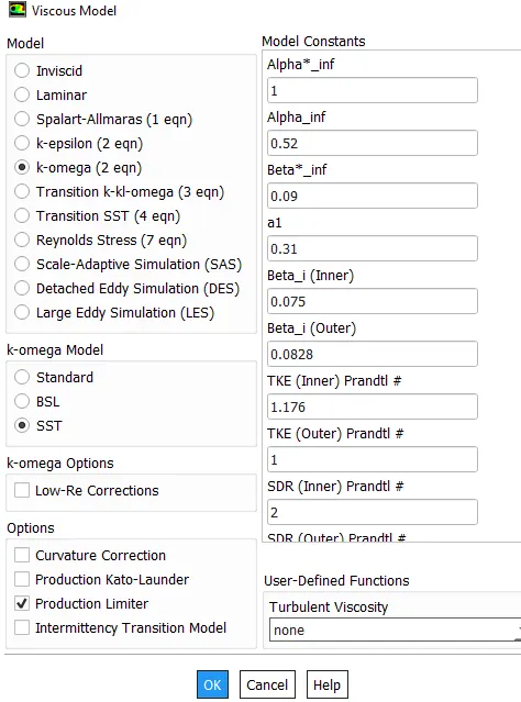
Fig No. 11. Viscous Model

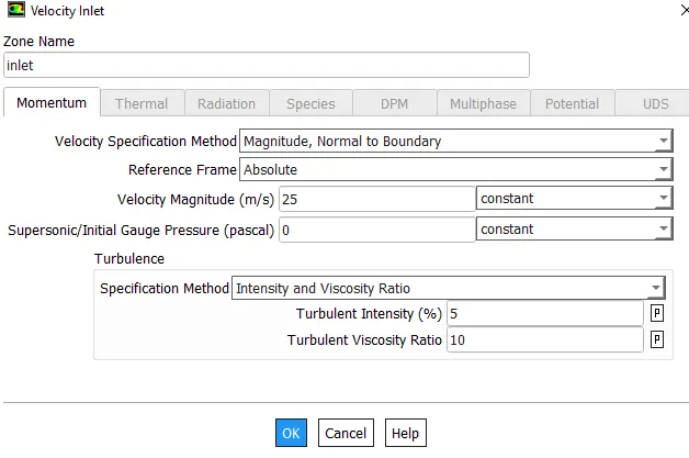
Fig No. 12. Velocity Inlet

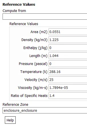
Fig 13. Reference Values.

--------------------------------------------------------------------------------------------------------------------------------------------

• Grid Independency Test -

Table No. 1 Variation in grids.

S.R. No.		FIRST	SECOND	THIRD	FOURTH	FIFTH
1.	OUTER ENCLOSURE	Multizone Size 0.1m	Multizone Size 0.1m	Multizone Size 0.1m	Multizone Size 0.1m	Multizone Size 0.08m
2.	INNER ENCLOSURE	Tetrahedral Size 5e-2 m.	Tetrahedral Size 5e-2 m.	Tetrahedral Size 4e-2 m.	Tetrahedral Size 3.5e-2 m.	Tetrahedral Size 3e-2 m.
3.	AHMED BODY	Face Size - 1e-2 m	Face Size - 1e-2 m	Face Size - 0.8e-2 m	Face Size - 0.8e-2 m	Face Size - 0.6e-2 m
4.	PILLARS OF AHMED BODY	Face Size - 5e-3 m	Face Size - 5e-3 m	Face Size - 5e-3 m	Face Size - 4e-3 m	Face Size - 2e-3 m
5.	INFLATION LAYER	1.426*10^-5 m
5.1	TOTAL THICKNESS	3.5483*10^-5 m	3.5483*10^-5 m	3.5483*10^-5 m	6.1315*10^-5 m	6.1315*10^-5 m
5.2	NUMBER OF LAYERS	6	6	6	9	9
5.3	GROWTH RATIO	1.2	1.2	1.2	1.2	1.2
6.	TOTAL NODES	109134	109304	167137	218786	431581
7.	TOTAL ELEMENTS	386571	387614	620403	759130	1451000

• CASE FIRST -

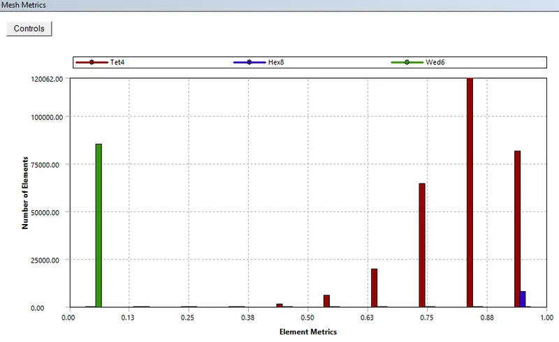
Fig No. 14. Element metrics.

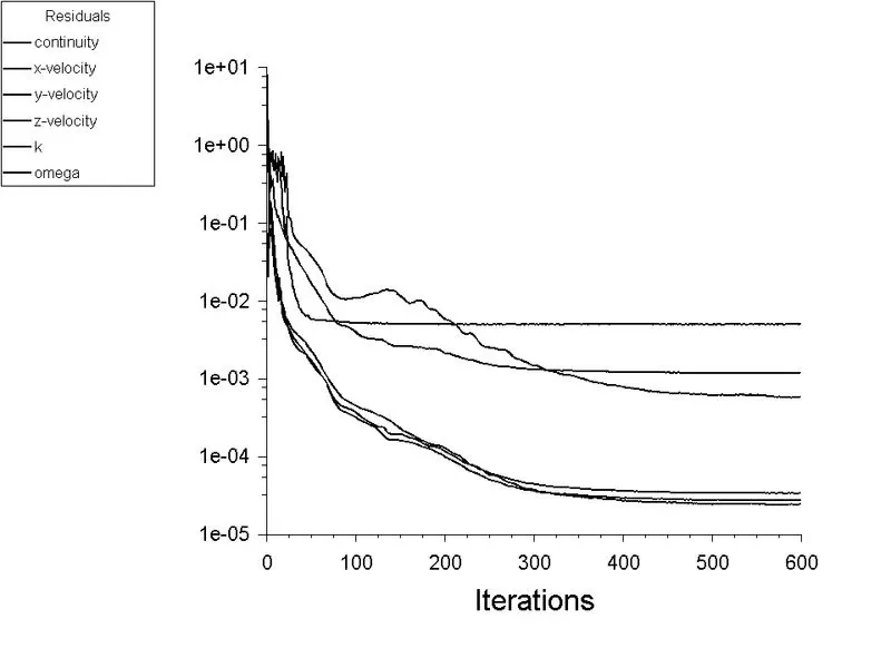
Fig No. 15. Residual

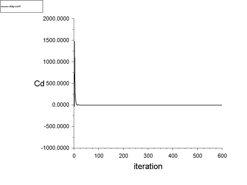
Fig No. 16. Coefficient of Drag.

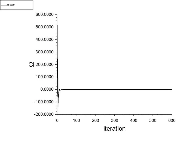
Fig No. 17. Coefficient of lift.

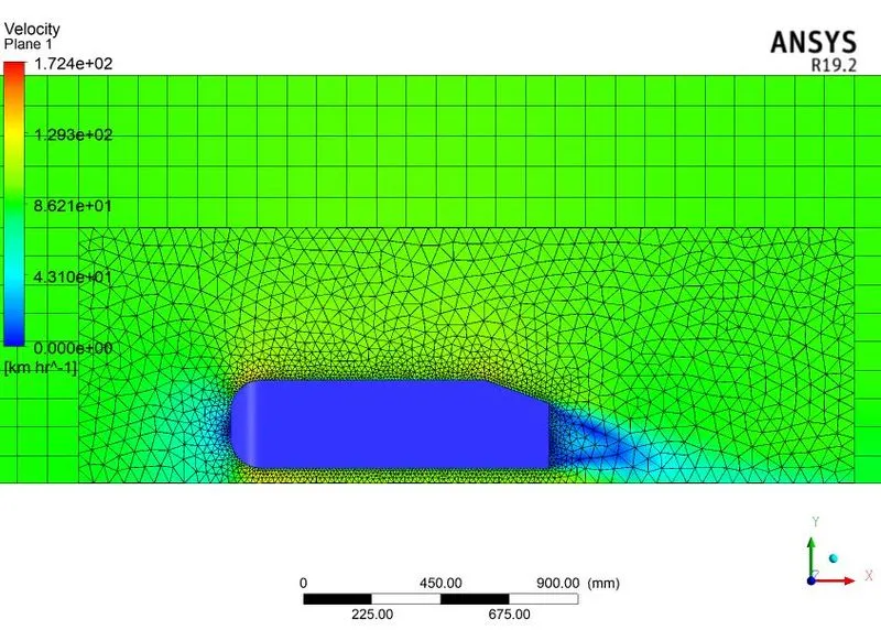
Fig No. 18. Velocity Contour on the plane.

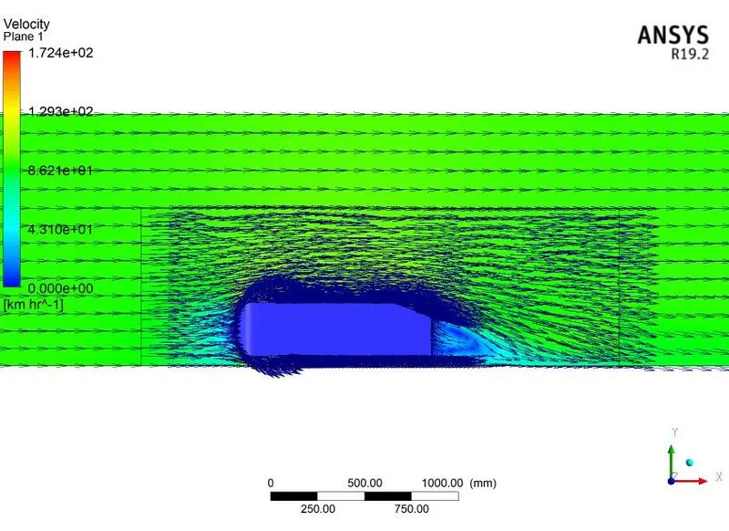
Fig No. 19. Velocity Vector plot.

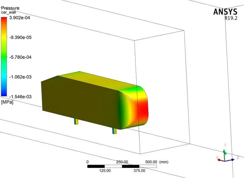
Fig No. 20. Pressure distribution over the Ahmed Body.

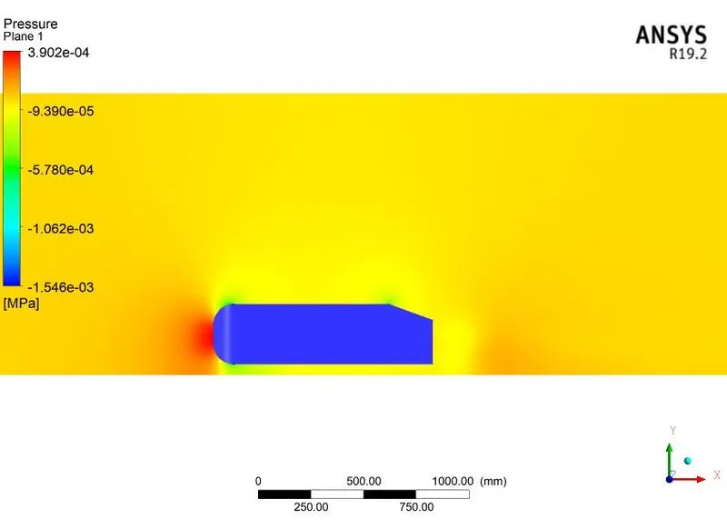
Fig No. 21. Pressure Contour over a plane.

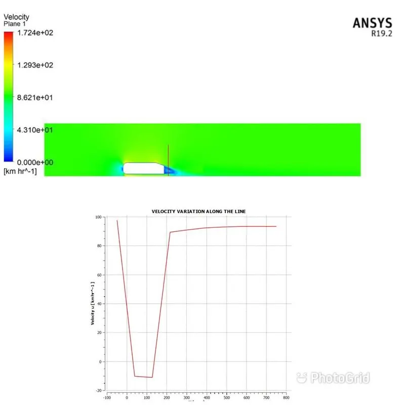
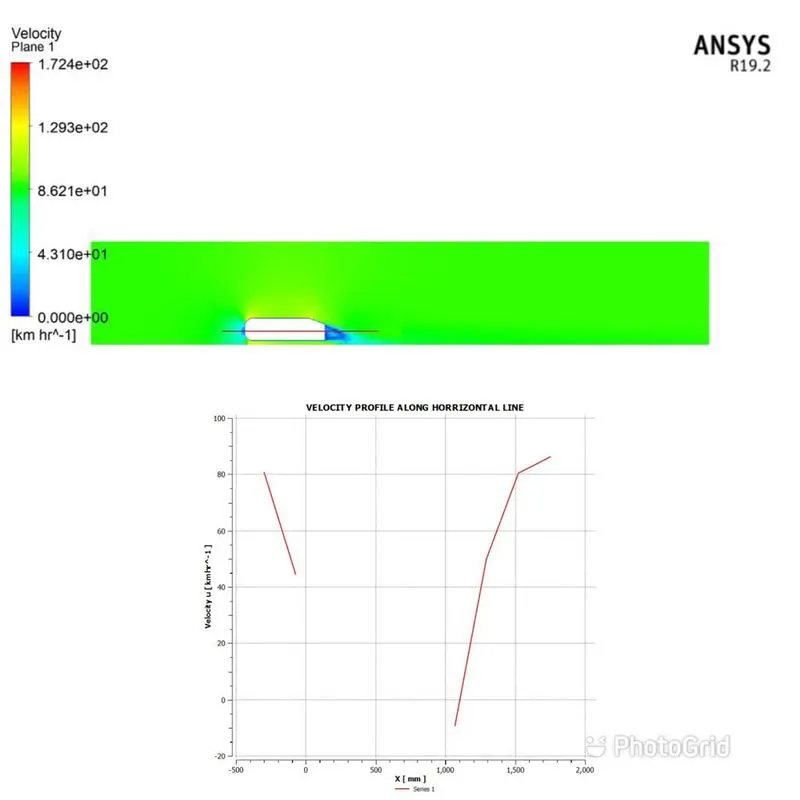
Fig No. 22. The graph plotted along the vertical and horizontal lines.

--------------------------------------------------------------------------------------------------------------------------------------------

• CASE SECOND -

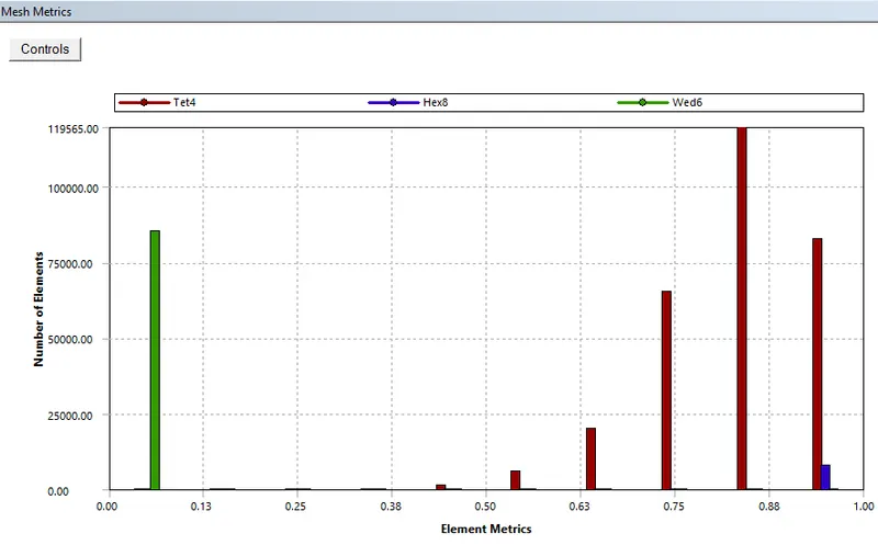
Fig No. 23. Element metrics.

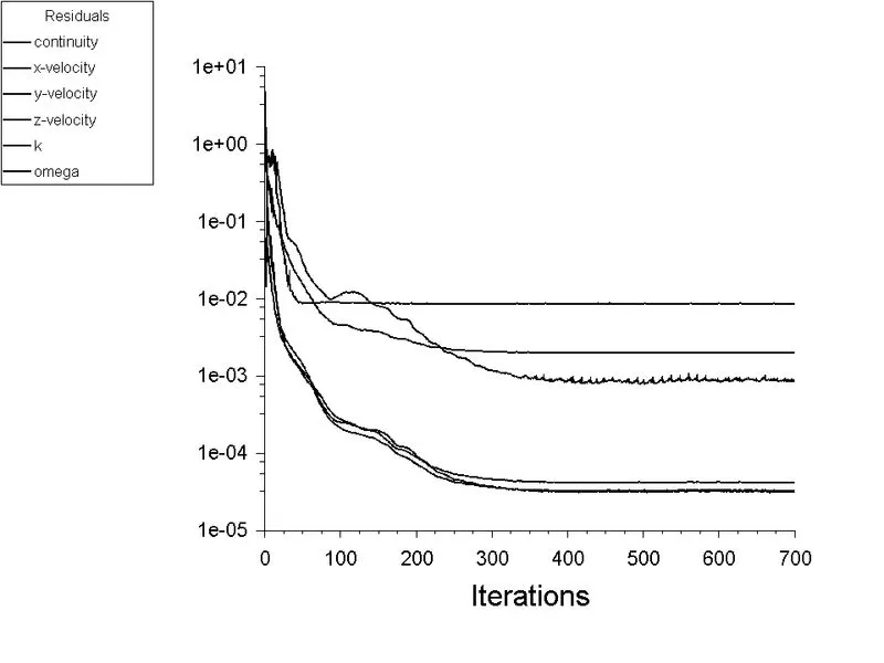
Fig No. 24. Residual

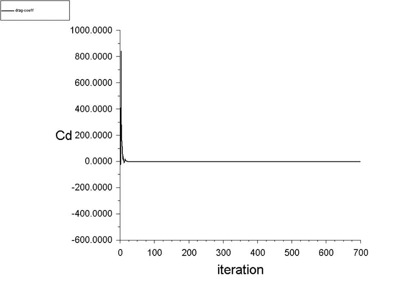
Fig No. 25. Coefficient of Drag.

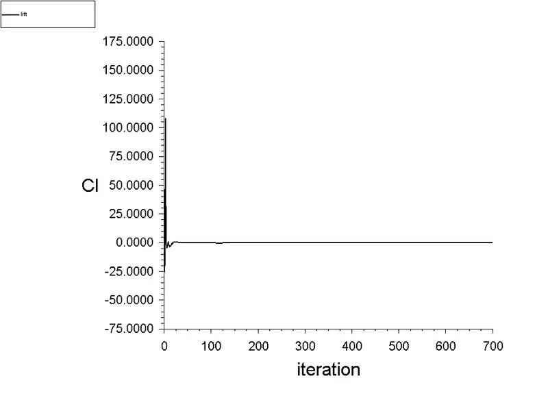
Fig No. 26. Coefficient of lift.

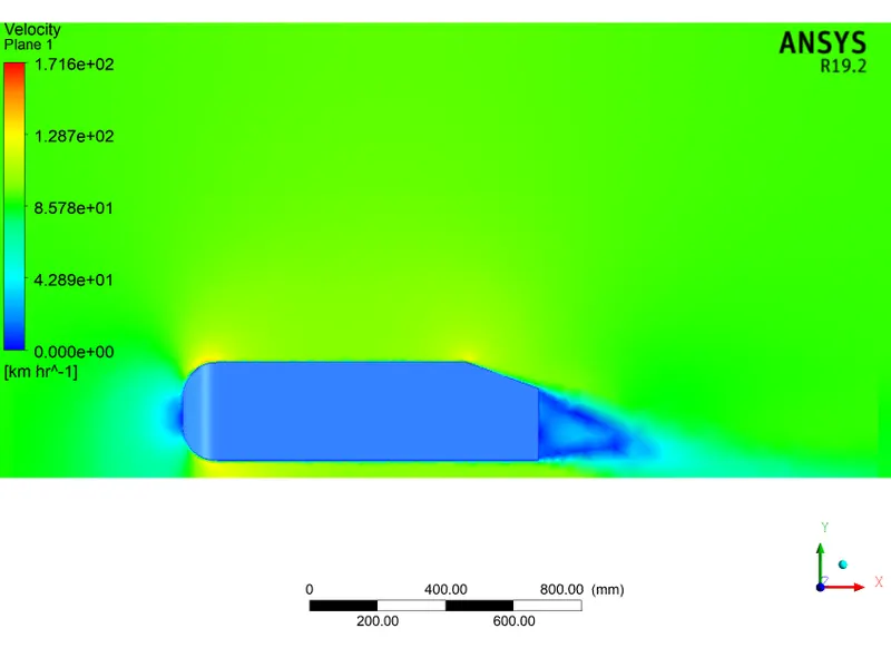
Fig No. 27. Velocity Contour on the plane.

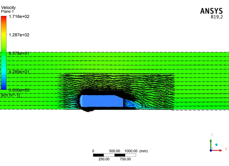
Fig No. 28. Velocity Vector plot.

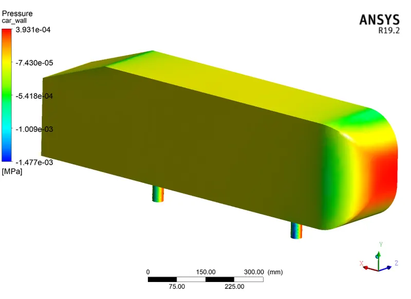
Fig No. 29. Pressure distribution over the Ahmed Body.

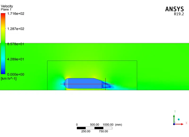
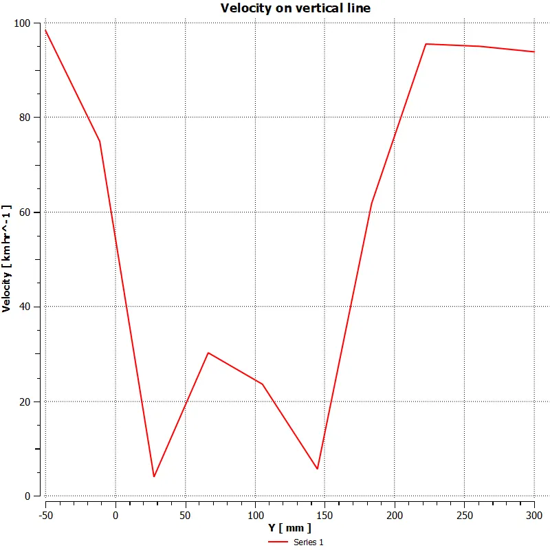
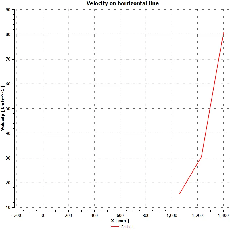
Fig No. 30. The graph plotted along the vertical and horizontal lines.

---------------------------------------------------------------------------------------------------------------------------------------------

• CASE THIRD -

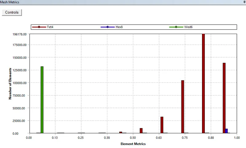
Fig No. 31. Element metrics.

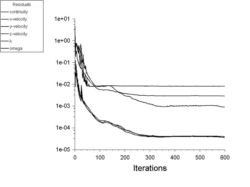
Fig No. 32. Residual

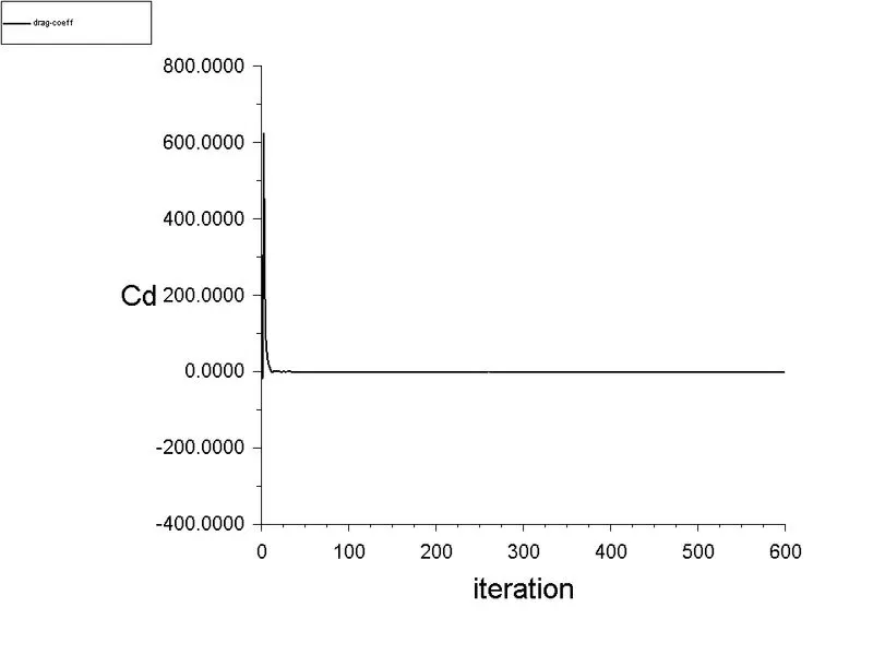
Fig No. 33. Coefficient of Drag.

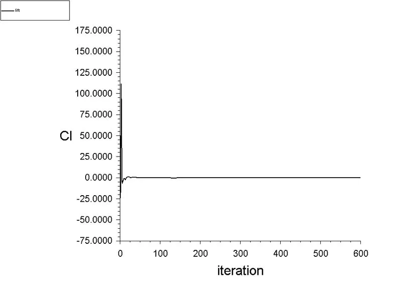
Fig No. 34. Coefficient of lift.

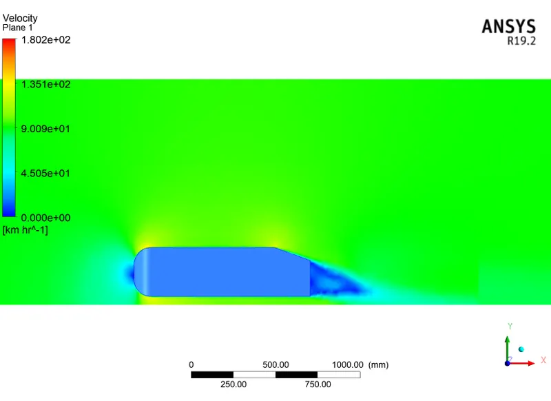
Fig No. 35. Velocity Contour on the plane.

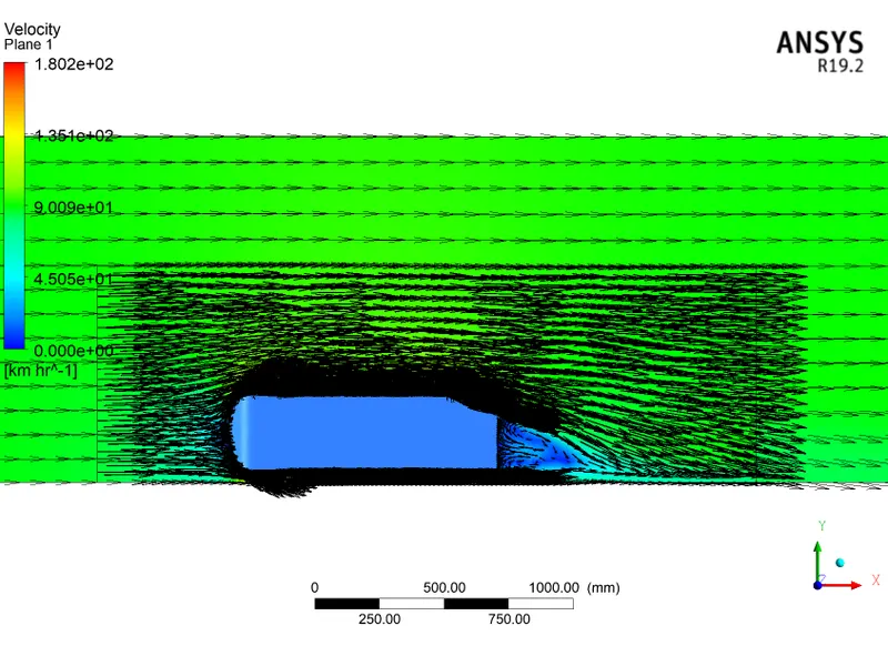
Fig No. 36. Velocity Vector plot.

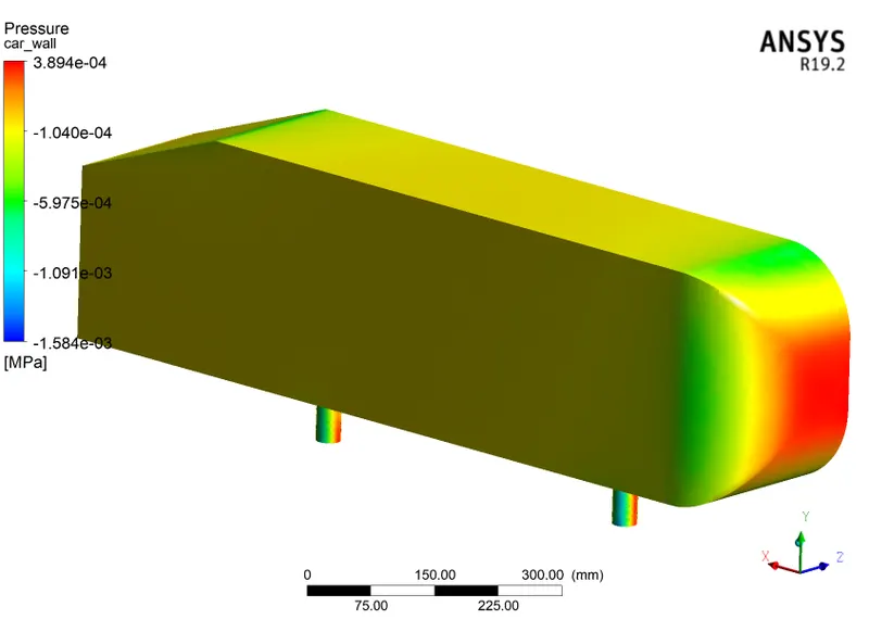
Fig No. 37. Pressure distribution over the Ahmed Body.

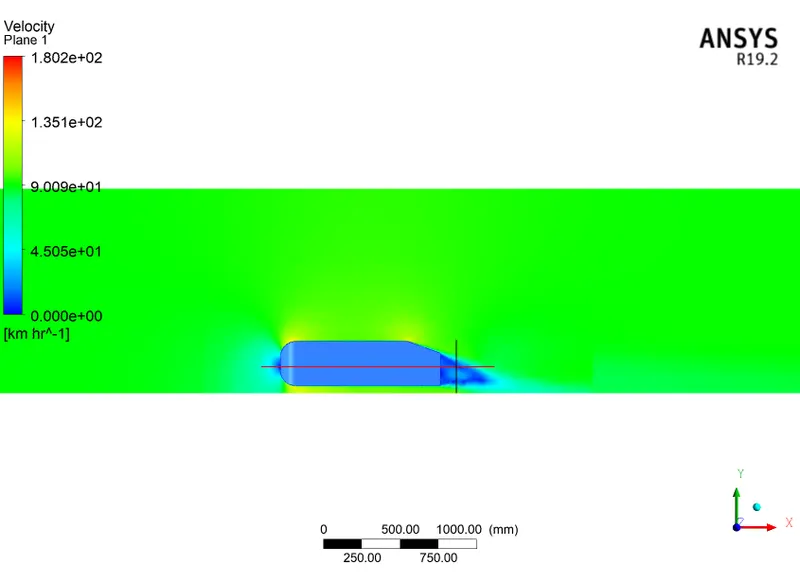
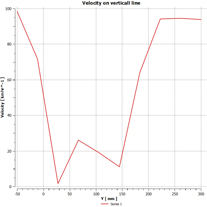
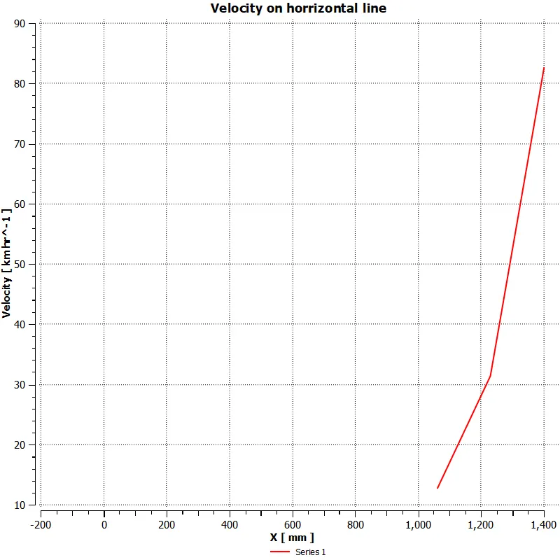
Fig No. 38. The graph plotted along the vertical and horizontal lines.

------------------------------------------------------------------------------------------------------------------------------------------------

• CASE FOURTH -

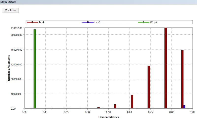
Fig No. 39. Element metrics.

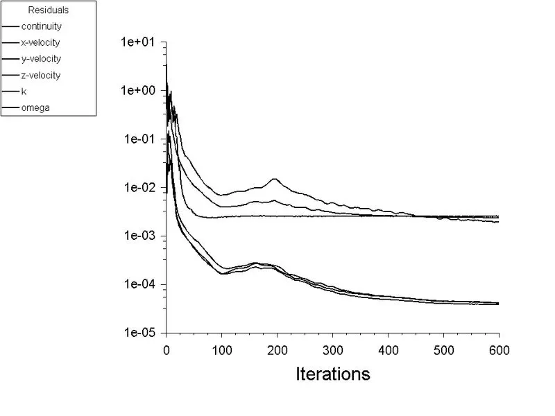
Fig No. 40. Residual

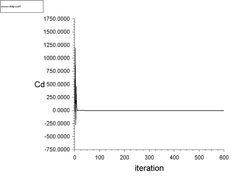
Fig No. 41. Coefficient of Drag.

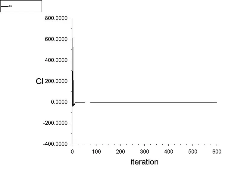
Fig No. 42. Coefficient of lift.

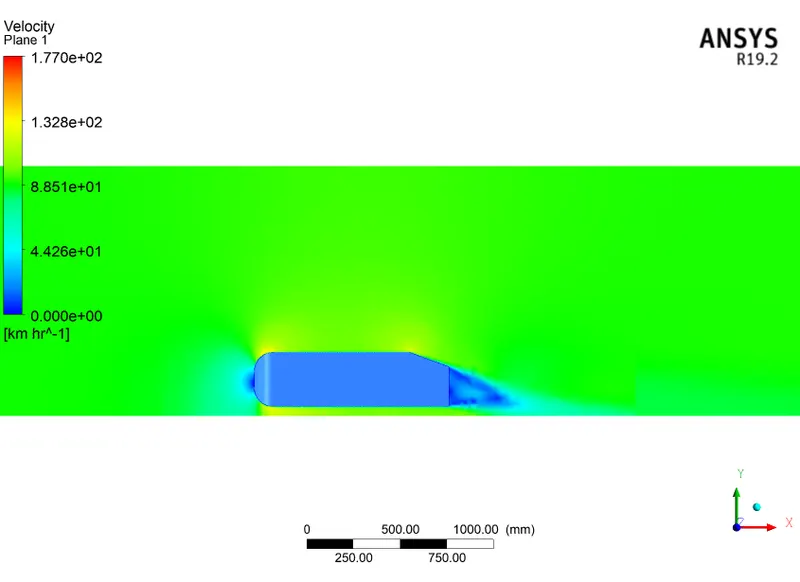
Fig No. 43. Velocity Contour on the plane.

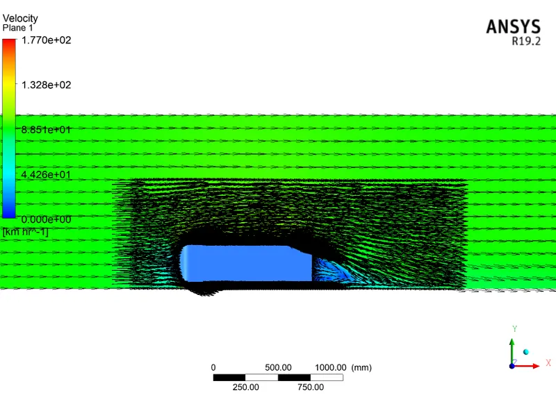
Fig No. 44. Velocity Vector plot.

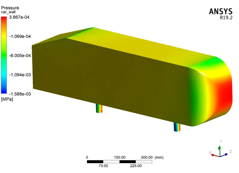
Fig No. 45. Pressure distribution over the Ahmed Body.

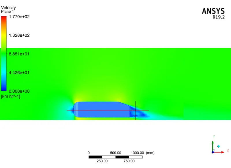
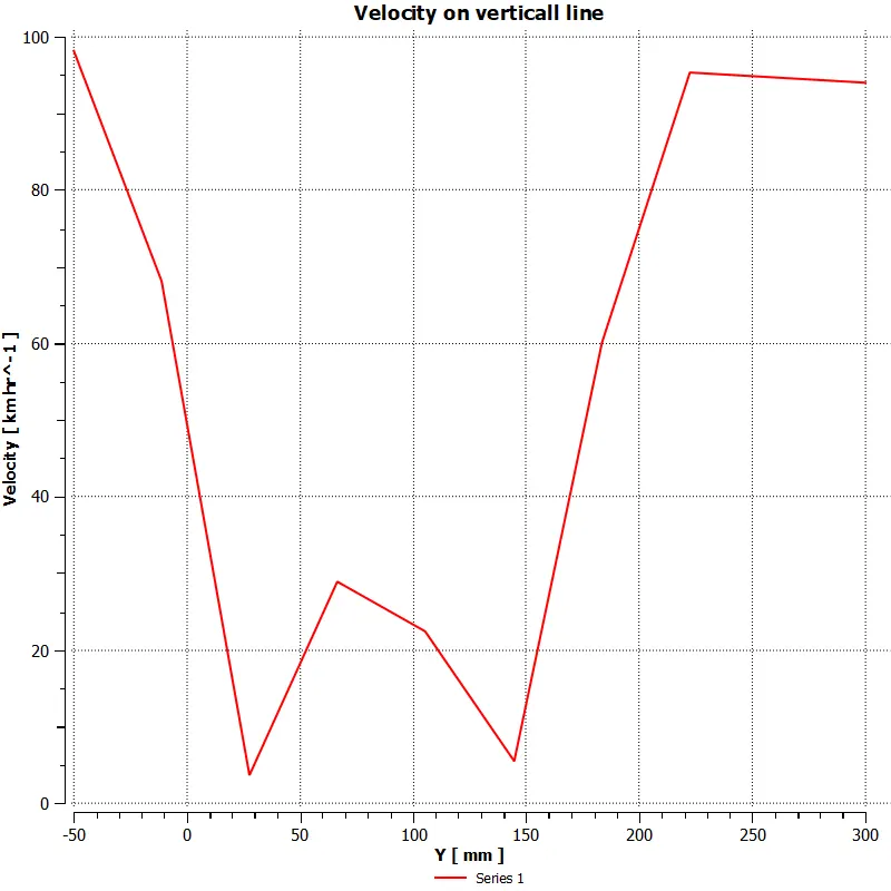
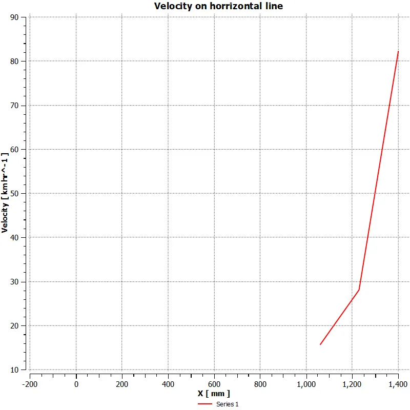
Fig No. 46. The graph plotted along the vertical and horizontal lines.

-------------------------------------------------------------------------------------------------------------------------------------------------

• CASE FIFTH - We move one step further and this time we are created a more dense mesh structure to observe the variation.

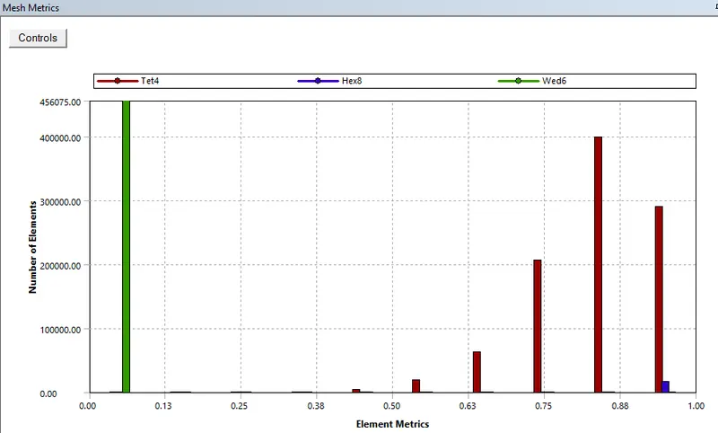
Fig No. 47. Element metrics.

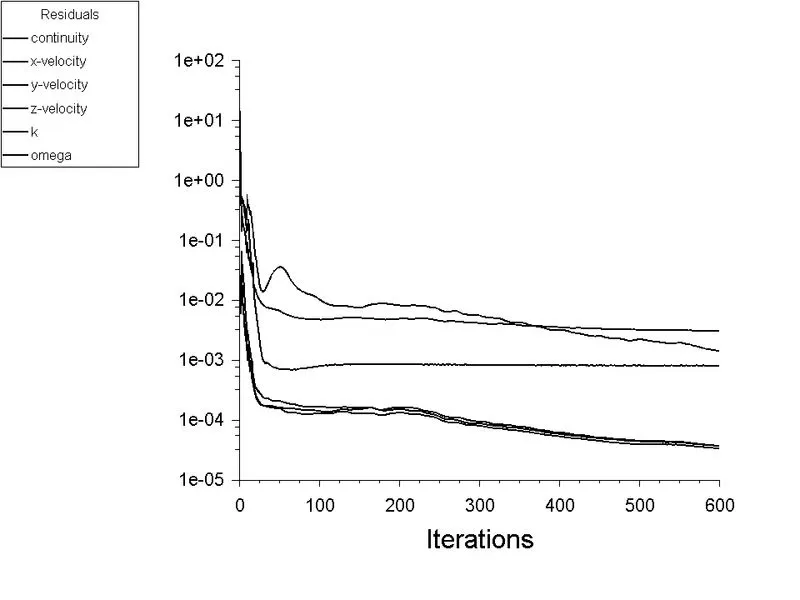
Fig No. 48. Residual

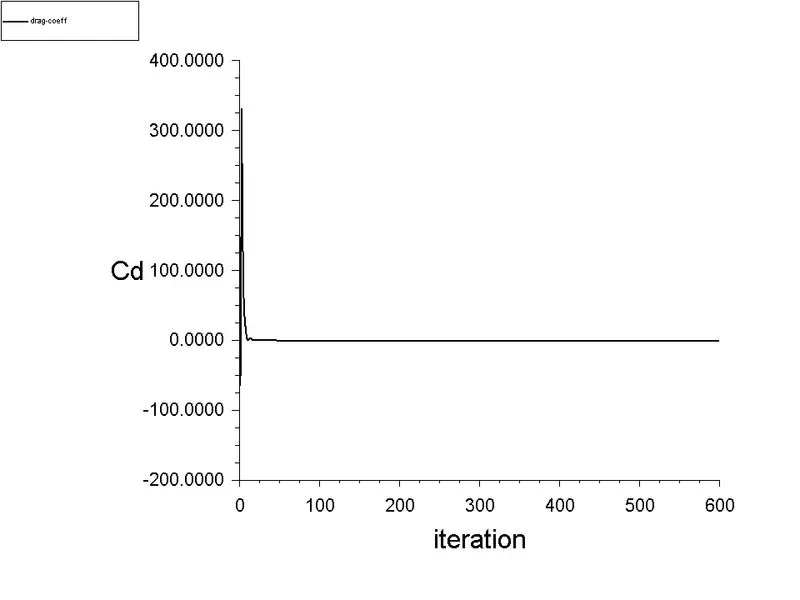
Fig No. 49. Coefficient of Drag.

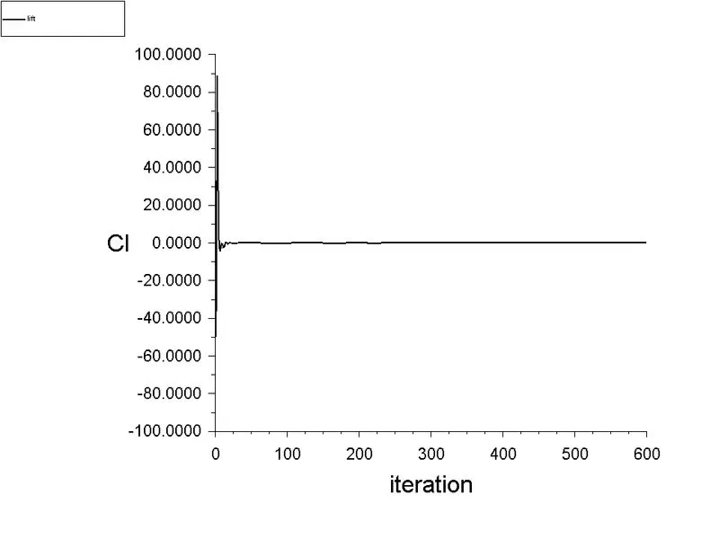
Fig No. 50. Coefficient of lift.

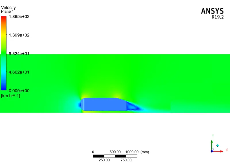
Fig No. 51. Velocity Contour on the plane.

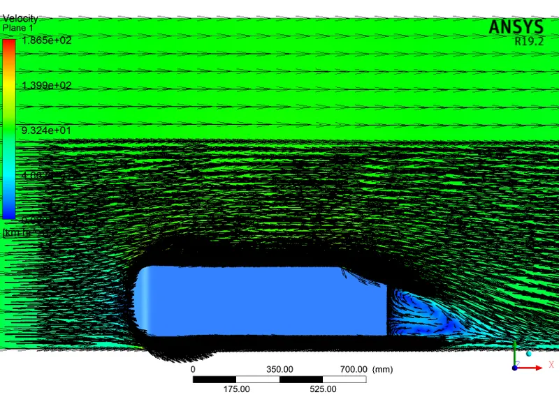
Fig No. 52. Velocity Vector plot.

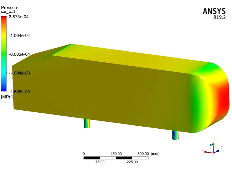
Fig No. 53. Pressure distribution over the Ahmed Body.

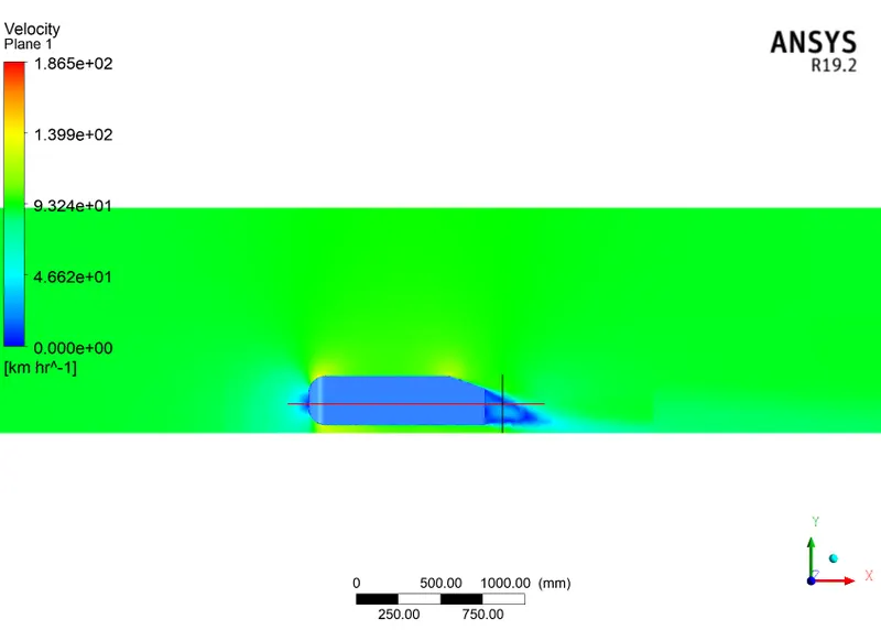
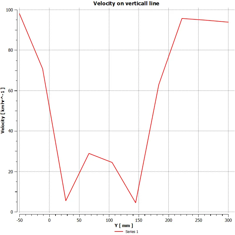
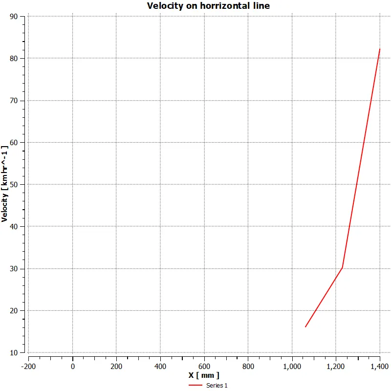
Fig No. 54. The graph plotted along the vertical and horizontal lines.

Table No. 2 Coefficient of Drag and lift.

S.R. No.		FIRST	SECOND	THIRD	FOURTH	FIFTH
1.	NODES	109134	109304	167137	218786	431581
2.	ELEMENTS	386571	387614	620403	759130	1451000
3.	COEFFICIENT OF DRAG	0.2809	0.3012	0.3217	0.3307	0.3321
4.	COEFFICIENT OF LIFT	0.2353	0.2458	0.2467	0.3487	0.3458

We can observe from various plots and charts the results do change majorly up to the third iteration but after the third case in case, four and fifth the variation in the results is small. As stated the coefficient of drag in the literature for standard Ahmed body by using wind tunnel testing found out to be 0.33 and after the fourth iteration, we are able to get the standard result of 0.33 in the coefficient of drag. In the final iteration, we get one step further and the mesh is so dense in the targeted areas. If we get more further dense structure then the variation in the results is comparatively negligible.

-----------------------------------------------------------------------------------------------------------------------------------------------

• NEGATIVE PRESSURE IN THE WAKE REGION -

A high-pressure region is observed in the front of Ahmed body and a drop in pressure is observed when the flow leaves the Ahmed body at the rear (As shown in Figures 20 and 21). This detachment of fluid at the rear results in eddy formation and disturbance in the flow. The region behind Ahmed body where the flow is unstable is called the wake, where pressure adversely drops.

At the inlet, fluid flows with the velocity of `Uoo = 25`m/s when it encounters the Ahmed body in front of it high-velocity fluid is stagnated and reduces velocity results in high pressure. The fluid that comes in contact with the body behaves like a viscous sublayer this property of fluid remains until it is in contact with the body. At the slant of Ahmed body flows pf fluid separates the body and point of separation occur.

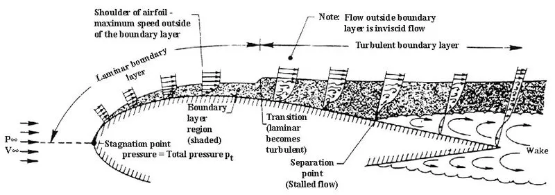
Fig No. 55. Boundary-Layer separation over the wing. Source: aerospaceengineeringblog.com

When fluid flows over the body, the boundary layer thickness increases. The fluid layer adjacent to the surface friction by consuming some kinetic energy. This loss of kinetic energy recovered from the adjacent fluid layer through the momentum exchange process. Thus the velocity of the layer goes on decreasing. Along the length of the body, at a certain point, a stage may come when the boundary layer may not be able to keep sticking to a solid body. The boundary layer will be separated from the surface. This phenomenon called boundary layer separation.

Near the surface of the solid when the point of separation occurs the fluid is incapable of sticking onto the surface. This arises the point where pressure reduces to negative. This induces extra drag force at the rear which creates a loss in the velocity of the fluid and reduces the velocity of the body. This negative pressure in the rear gives rise to vortices and eddies which creates losses. So for that reason in most cases the point of separation of the boundary layer designed in such a manner as to create the negative pressure away from the boundary.

Table No. 3. Conditions of Boundary-Layer separation

	Pressure Gradient	Velocity Gradient
Boundary layer separation does not occur	`(delp)/(delx)<0`	`(delu)/(dely)>0`
On the verge of separation (Point of separation)	`(delp)/(delx) = 0`	`(delu)/(dely) = 0`
Boundary layer separation occur	`(delp)/(delx)<0`	`(delu)/(dely) < 0`

`(delp)/(delx) > 0` when P1 is less or negative in manner with P2.

• SIGNIFICANCE OF THE POINT OF SEPARATION -

The point on the body where the boundary layer lifts off the surface is called the separation point. When the airflow separates off the surface, the pressure drag usually increases. The separation point is the point where the air stops "sticking" to an object that is moving through the air. When an object is moving through the air, the air molecules push back on it and resist the object's movement - this resistance is called pressure drag.

The position of the point of separation plays an essential role in the case where one wants less aerodynamic drag. To achieve this we can find several examples that are implemented in recent years the continuous shape of an outer layer of the body, providing wings, flaps, slats to locate the point of separation away from the body. The arrangements changes from application to application but the basic idea behind it is to reduce the drag as much as possible and make the object aerodynamically stable. After the point of separation from the figure, the formation of eddies is started.

• CONCLUSION -

1.The grid independency test is carried out to demonstrate the variation of the result with respect to the accuracy of the mesh. The need for a good quality mesh to achieve an accurate result.

2. The need of choice of Y+ according to application and quality of result need to attain by calculating the y value. The value of the coefficient of drag primarily depends upon the accurate value of Y+ in such cases grid independency test plays an important role.

3. In the boundary layer separation, the need of the correct location of the separation point while designing for the vehicle.