Mixing efficiency

MIXING TEE EFFECTIVENESS

AIM - IN STEADY STATE SIMULATION TO STUDY THE EFFECTIVENESS OF FLUID AT T JUNCTION HAVING DIFFERENT TEMPERATURE, ANALYZING DIFFERENT PARAMETERS AFFECTING IN MIXING USING ANSYS FLUENT 19.2.

INTRODUCTION -

Computational fluid dynamics model developed using ANSYS Fluent to study the effectiveness of mixing tee, in this model the hot and cold fluid are mixed with each other. In mixing tee by varying the length of pipe and velocity of cold fluid by changing the momentum ratio of the fluid behavior is observed. Different cases have been developed to study the behavior changes in mixing tee. In this study, the results are analyzed by checking how properly fluids are mixing. k epsilon and k omega models are compared to decide the result variation, both models are used for turbulence modeling. k omega model and k epsilon model have their advantages according to applications. The effectiveness of mixing is varied mainly with the length of pipe and momentum ratio, by changing each parameter how they affect in both models is analyzed.

Mixing of fluid having different velocities and temperature is observed in most of industrial as well as day to day basis. In day-to-day practice in houses such applications in the form of refrigerations, air conditioning, etc. similarly in industrial applications it has different kinds of applications from mixing of melted metals to all the way up to mixing of fluid in a nuclear power plant. The study is a basic platform for understanding and formulation for different applications.

• Geometry -

The CFD simulation basically starts with modeling of the TEE in CAD software. It is not necessary always to use such complex geometry. So interested volume areas have been extracted as shown below. In this case, the external shell has been suppressed and internal volume extracted.

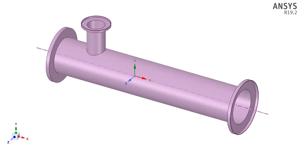
Fig 1. Solidworks Geometry

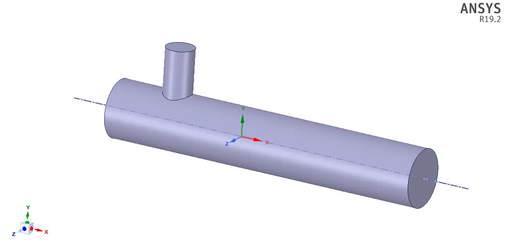
Fig 2.Volume extracted

Geometry details - It is tabulated as below in LONG and SHORT pipes format and differences:

TABLE 1. Geometry details

PIPES LENGTH	Volume (m^3)	Average Surface Area (m^2)
long	1.7944e-4	4.7397e-3
short	2.4796e-4	6.3528e-3

In the above, images show that the volume extraction from the CAD model. It reduces the time required to solve the domain by simplifying geometry.

• MESHING -

In this study, we majorly carrying out study for two cases LONG and SHORT pipes. Furthermore, these cases are subdivided into subcases based on the momentum ratio and model used for solving.

Now, in meshing it is classified as LONG and SHORT pipes. In this case, focused on the quality mesh and comparison of mesh based on different parameters.

• SHORT PIPE -

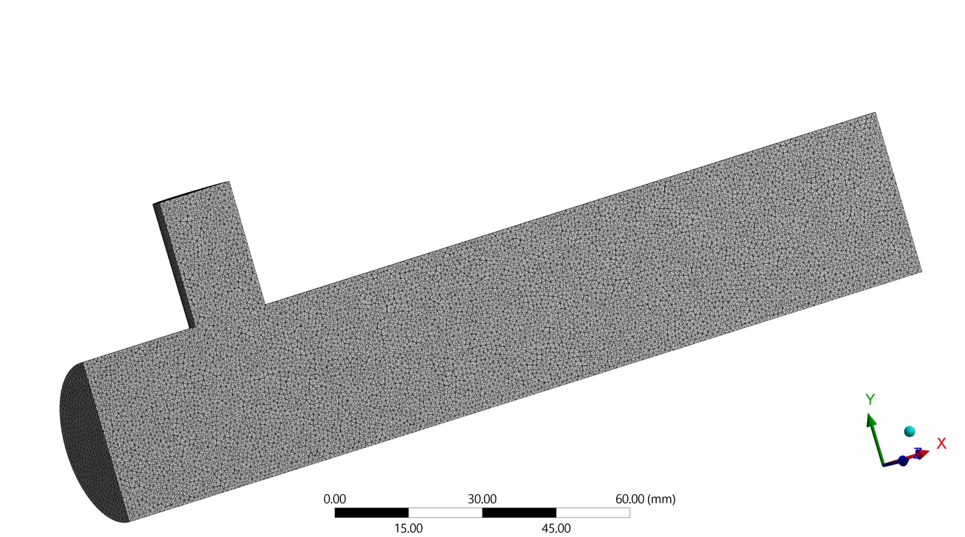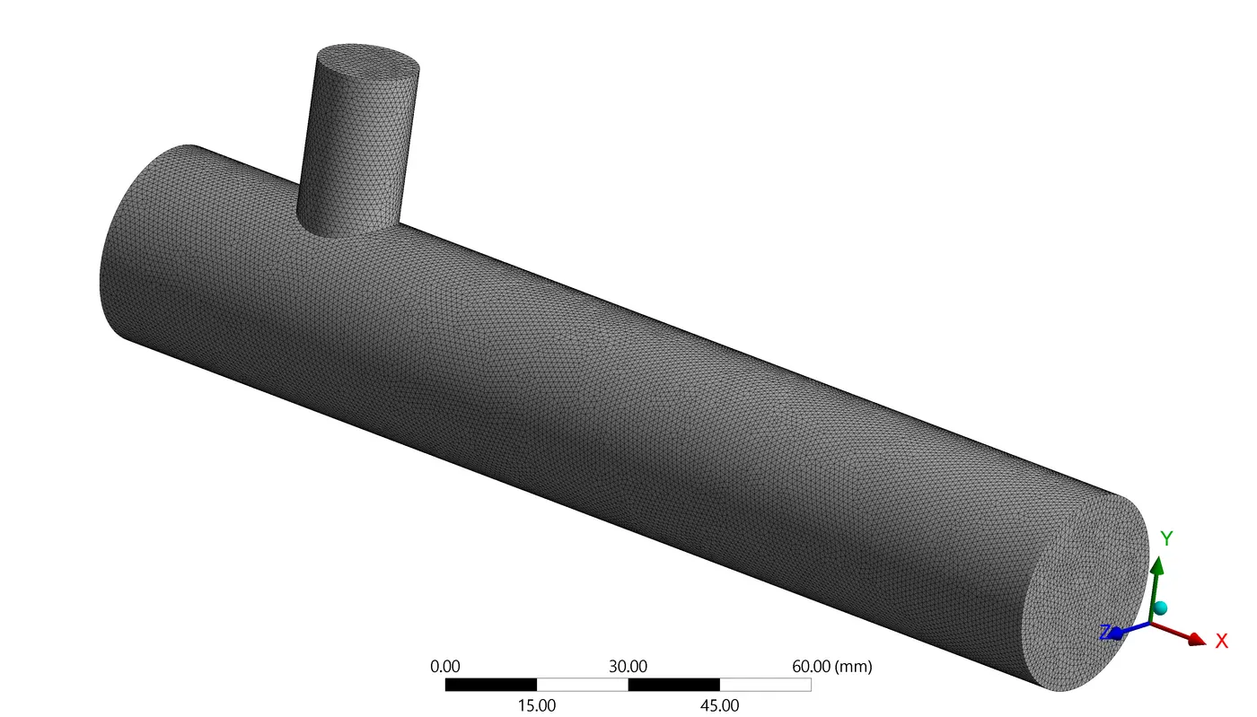
Fig 3. Meshed and cut section of geometry

The domain of working of the study is basically is an inner section i.e. extracted volume so in that case, the main focus is to improve the meshing at an inner level of the pipe. So that growth rate and refinement are the parameters in focus.

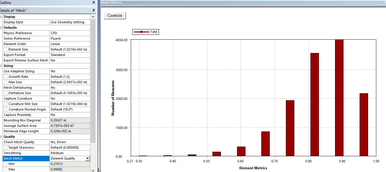Fig 4. Bounding box and mesh matrix chart for element quality

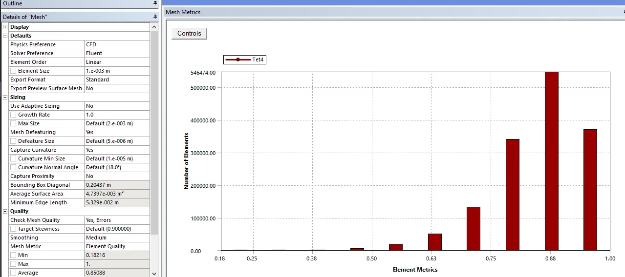Fig 5. One mm mesh with growth rate 1 and mesh matrix chart for element quality

In Figures 4 & 5, we can observe the increase in the number of nodes and mesh quality. The results are improved by step by step reducing the mesh size as well as changing the different parameters. By improving the mesh quality results quality also going to improve and contour is refined. The mesh results effect mostly on the results so enough importance and time should be given to improve the mesh quality.

Table 2. Element details in Short pipe

Element Size	Nodes	Elements	Convergence (Iterations)
The bounding box (Default)	892	406	145
5 mm	9428	5132	168
3 mm	27971	15759	172
1 mm (Growth rate = 1)	277236	161414	189
1 mm (Growth rate = 1, resolution 4)	324386	218191	198

The above table shows the mesh independent study and variation of different parameters and the changes in nodes and elements accordingly. In these cases, the convergence iterations are calculated and the number of iterations is increased. The result visualization and accuracy depend upon mesh density so that a 1 mm mesh chosen for further study.

• LONG PIPE -

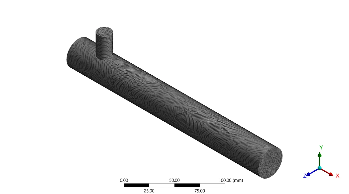
The area of interest is the inner surface and extracted in this case and then meshing is carried out.

Fig 6. Meshed and cut section of geometry

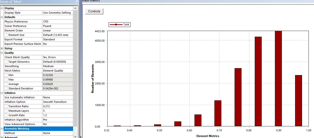Fig 7. Bounding box and mesh matrix chart for element quality

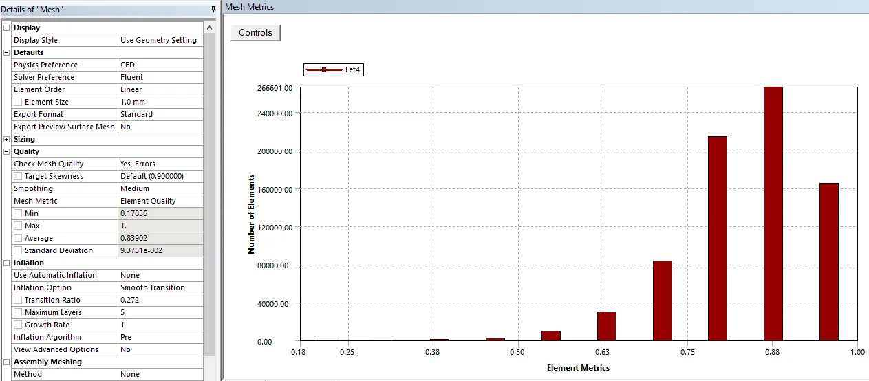Fig 8. One mm mesh with growth rate 1 and mesh matrix chart for element quality

The above figure shows the mesh matrix for element quality. The results depend upon the quality of mesh and mesh depends upon various parameters.

Table 3. Element details in Short pipe

Element Size	Nodes	Elements	Convergence (Iterations)
The bounding box (Default)	1263	619	128
5 mm	6831	3684	165
3 mm	20171	11334	178
1 mm (Growth rate = 1)	201551	117457	196
1 mm (Growth rate = 1, resolution 4)	275250	172074	202

In the table, in mesh independent study it shows that by changing mesh size, growth rate, and refinement parameter increase in the number of elements and nodes. The results are converged based on the above parameters of the meshing. As per the mesh size, increases iterations required for convergence also increases, and by reducing mesh size accuracy of the result increases.

• CFD MODEL SETUP -

In CFD simulations, the problem statement and its correct modeling play a very crucial role. The problem statement must consider interested aspects and focuses on real-time behavior. The logic behind starting such a problem is very necessary. Due to this reason, choosing correct models and having proper knowledge of models provided by the software is very much necessary. In our study, we mainly counter with k-epsilon Realizable model and k-omega SST model. According to the application shortlisted the model and both model satisfy for our study.

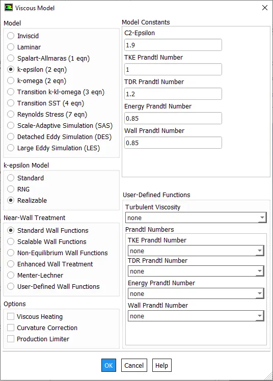Fig 9. Setup file model selection panel

As per the problem statement, a short pipe with 2 momentum ratio problems is solved by using both k-epsilon and k-omega SST models, and by comparing both results one of them is used for further cases and subcases. In comparing different contours, convergence and mixing effectiveness is observed.

Cell zones - It is used to decide the volume flow of the fluid and material selection of fluid. In our problem, we used air as a fluid for solving the mixture's effectiveness. In this problem, the material of fluid properties is tabulated in the below table are used. The behavior of the simulation largely depends upon the fluid that is going to use and it varies from fluid to fluid. The selection of fluid decides the results of simulations.

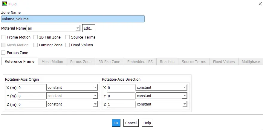Fig 10. Cell zone volume

Table 4. Air Fluid properties

Fluid	Mass flow rate (kg/m^3)	Cp (J/KgK)	Thermal conductivity	Viscosity
Air	1.225	1006.43	0.0242	1.7894e-5

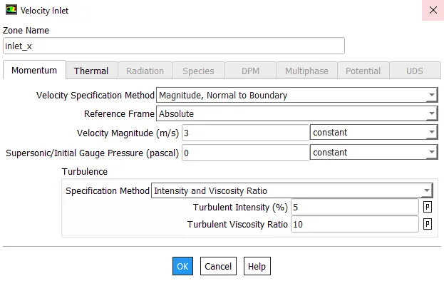
Hot fluid velocity and temperature are provided as input by using the following pannel. In this study, there are two inlets one with hot and another one with cold nature velocity of the fluid have been provided in momentum ratio. By varying these values one can easily change the behavior of the mixture fluid. Momentum ratio is basically the ratio of the hot fluid with respect to the cold fluid. The inlet velocity of the fluid is constant throughout the study which is 3m/s.

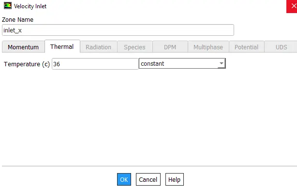Fig 11. Hot fluid velocity and temperature

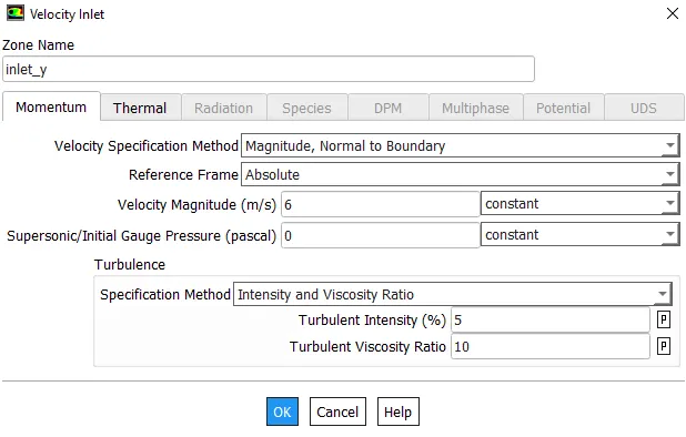
In the second inlet inputs values regarding the velocity and temperature of the cold fluid are substituted which are calculated by using the momentum ratio. The hot fluid velocity is constant but the velocity of cold fluid varies with momentum ratio from 2 and 4. The temperature of cold fluid is constant at 19C and the effect of mixing is observed in this study.

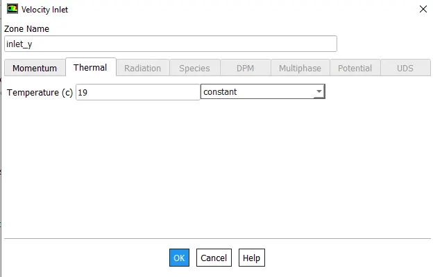Fig 12. Cold fluid velocity and temperature panel

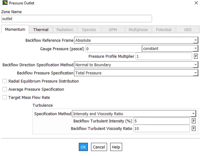Fig 13. Pressure outlet parameter

The remaining setup details and parameters are listed below, most of the values are keep default such as the no-slip boundary condition because that condition not going to affect majorly in this case. The momentum ratio is also defined in the below table.

Table 5. Setup boundary details

WALL	Stationary wall No-slip boundary Roughness constant = 0.5
OUTLET	Gauge pressure = 0 Back flow turbulent intensity = 5% Back flow turbulent viscosity ratio = 10
MOMENTUM RATIO	`(Hot fluid)/(Cold fluid)=2,4`

Lastly, the solution method needs to specify to solve the governing equations in matrix form. The appropriate solution method needs to decide, the convergence, results, and effectiveness depend upon the solution method.

Table 6. Solution Methods

Scheme	Simple
Gradient	Least squares cell-based
Pressure	Second-order
Momentum	Second-order upwind
Turbulent kinetic energy	First-order upwind
Turbulent dissipation rate	First-order upwind
Energy	Second-order upwind

• RESULTS -

The results are observed in two cases short pipe and long pipe, mixing effectiveness in this study depends upon the length of the pipe and velocity of the fluid. Based on the length two cases are created one with short and other one is long. these cases are subdivided into two types based on momentum ratios like 2 and 4. The results are tabulated and represented in a proper format.

• Short pipe momentum ratio 2 -

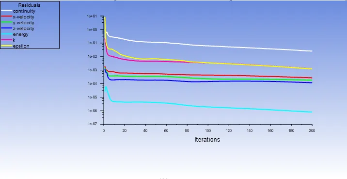
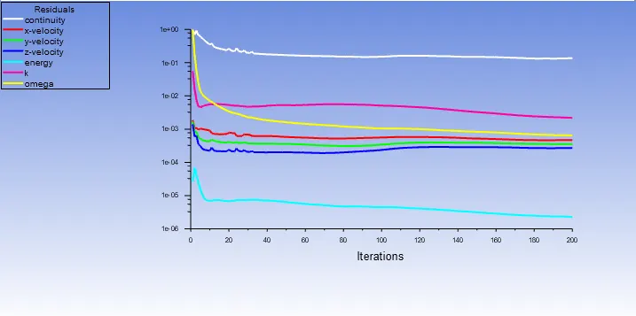
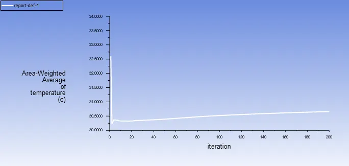
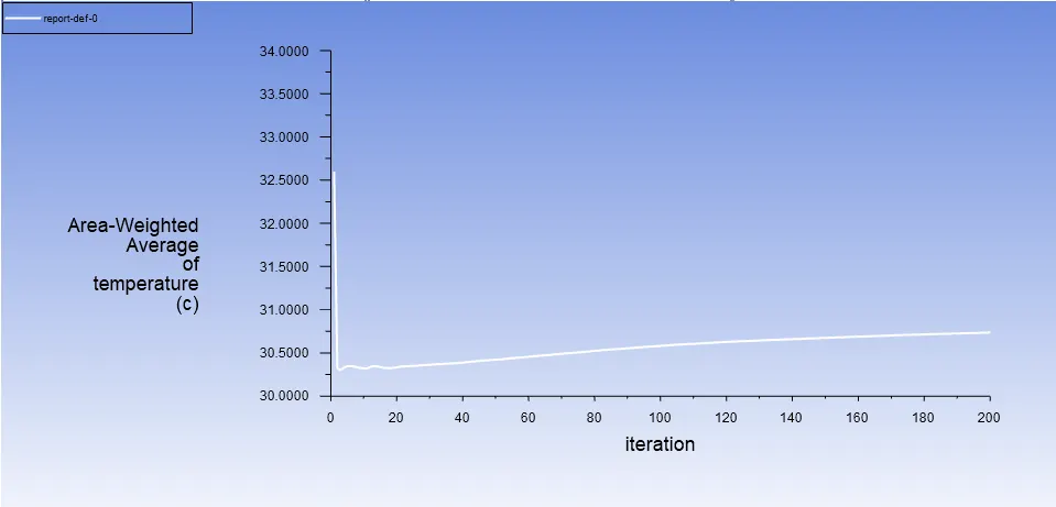
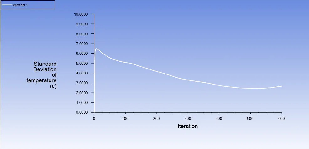
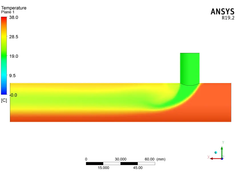
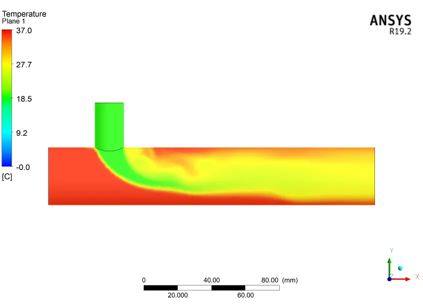
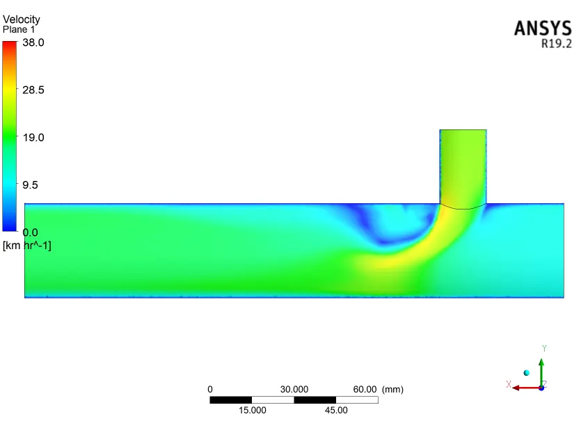
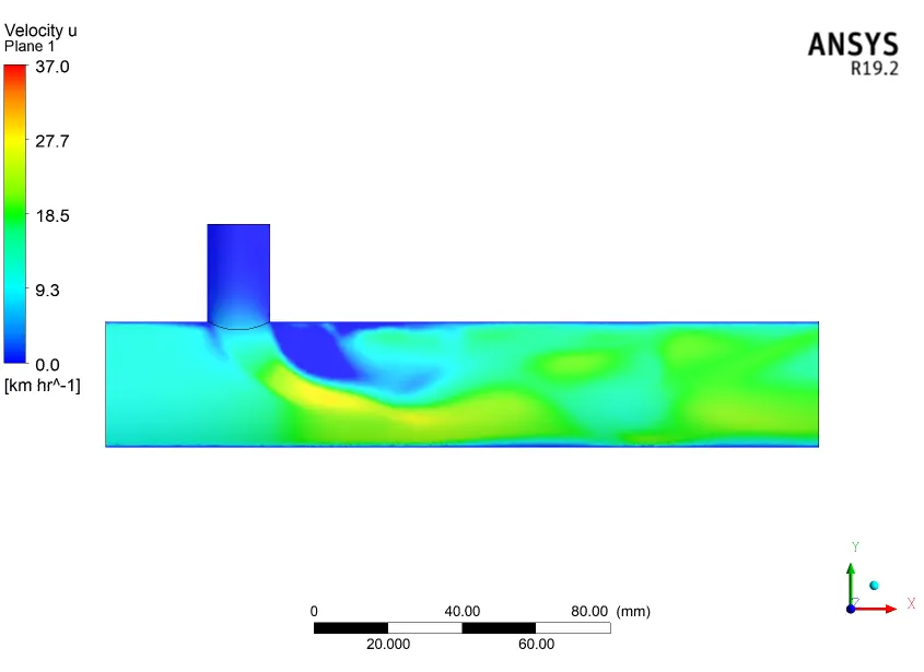
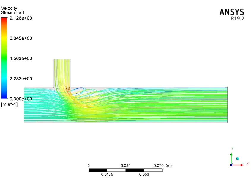
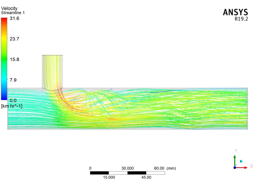
The decision of selecting a proper model for solving is always a crucial role. In most cases, the decision has been made by actual simulating results comparing it and then implementing it for further study. In our case below table shows different important parameters compared and later on based on that model has been selected.

K Epsilon realizable model	K omega SST model
It is a general description model with two transport equations used in turbulence modeling. It shown to be reliable for free shear flows such as one with low-pressure gradients. K epsilon model is used for predicting the behavior of fluid away from the wall.	SST K omega model is two equations eddy viscosity model that is used for many aerodynamic problems. SST model is used for simulating flow near the viscous sublayer i.e it can be used for flows with low Reynold number where the boundary layer is relatively thick. Thus k omega is better for near-wall treatment.

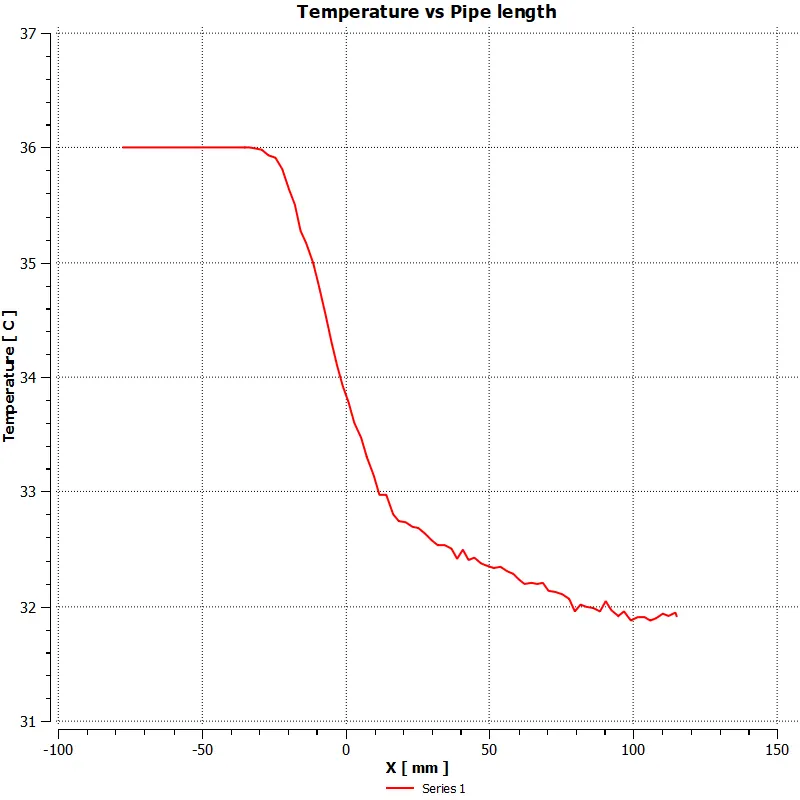
K epsilon is showing better results in the mixing area as compared to k omega though it is stated that K omega provides better prediction of flow separation and better near-wall treatment. On the negative side of K omega, this model produces large turbulence levels in the region with large normal strain and region with strong acceleration. So for further study, the K epsilon model is chosen and implemented.

• SHORT PIPE WITH MOMENTUM RATIO 4 -

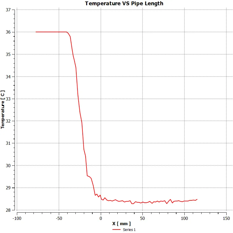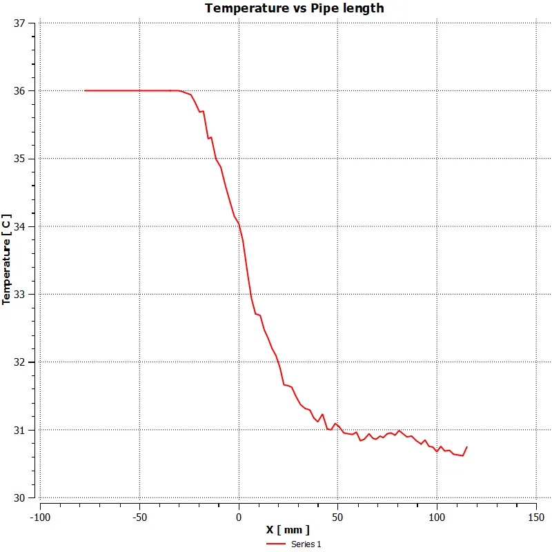
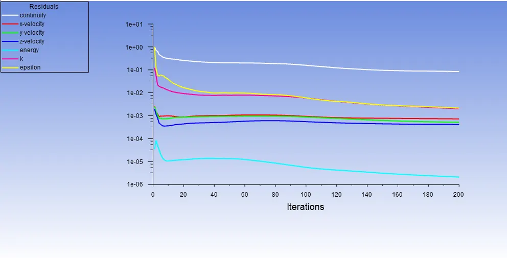
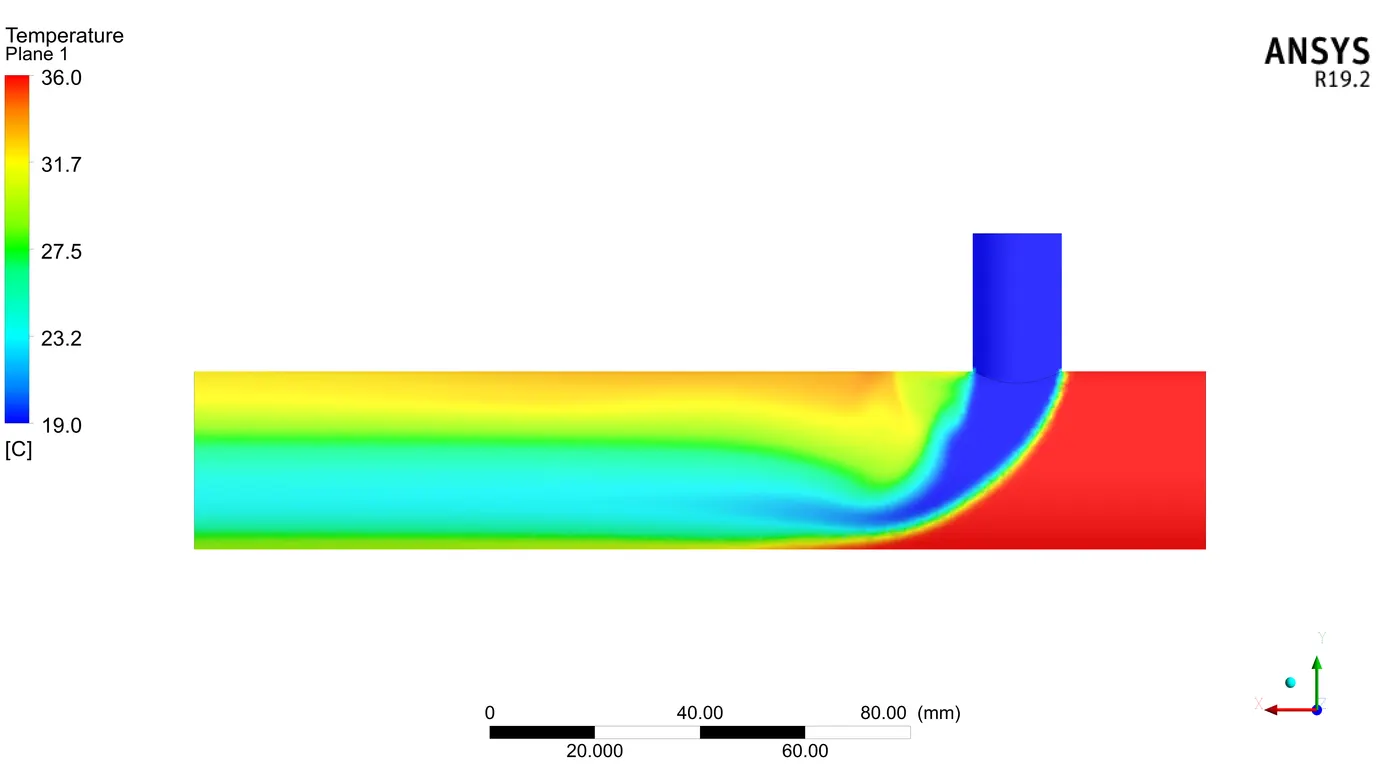
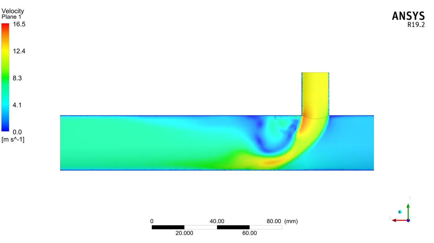
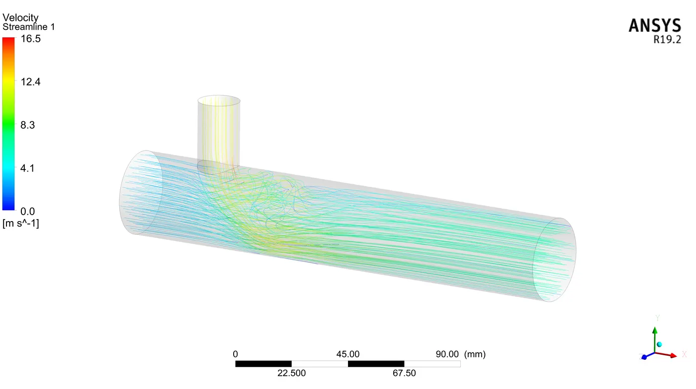
By increasing the momentum ratio, the fluid mixes very much properly as compare with the less momentum ratio. In the contour plot how well the fluids are mixed is clearly seen. In the graph variation of temperature and achieving stability, in the end, is observed. The streamlines are clearly observed and analyzed the result. The chart shows the stability in temperature along the length of the pipe.

• LONG PIPE WITH MOMENTUM RATIO 2 -

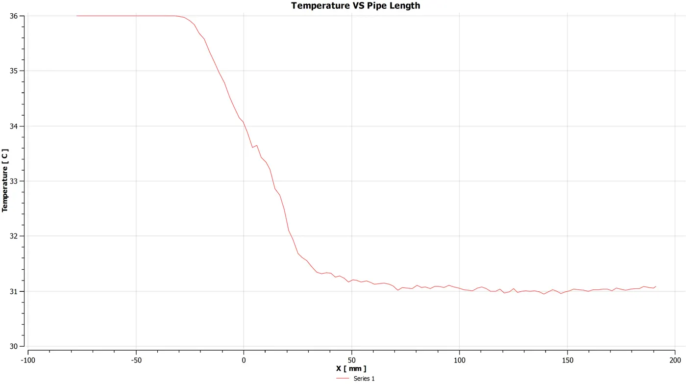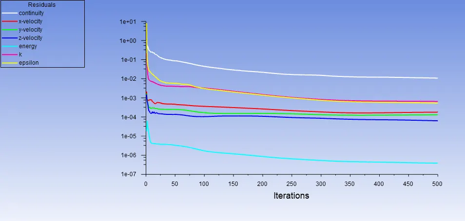
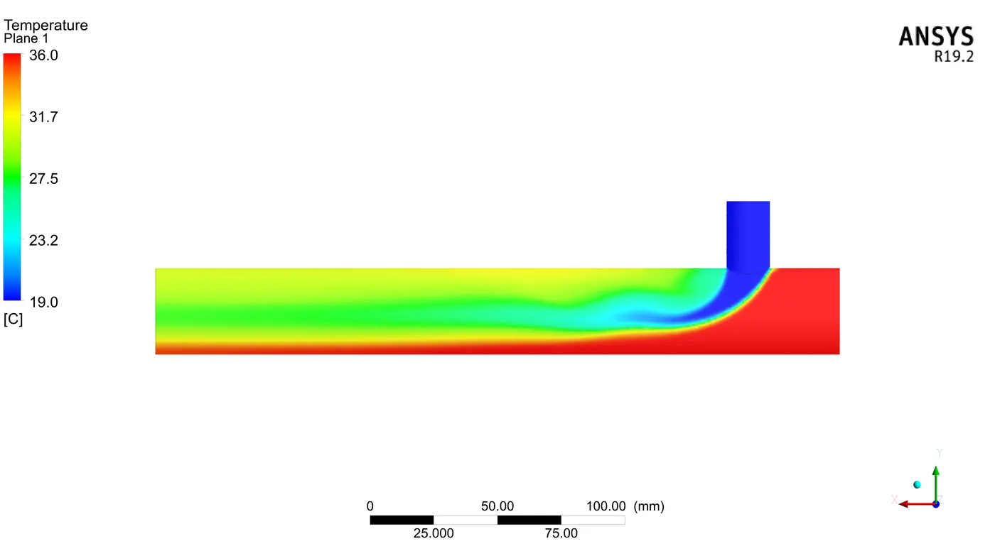
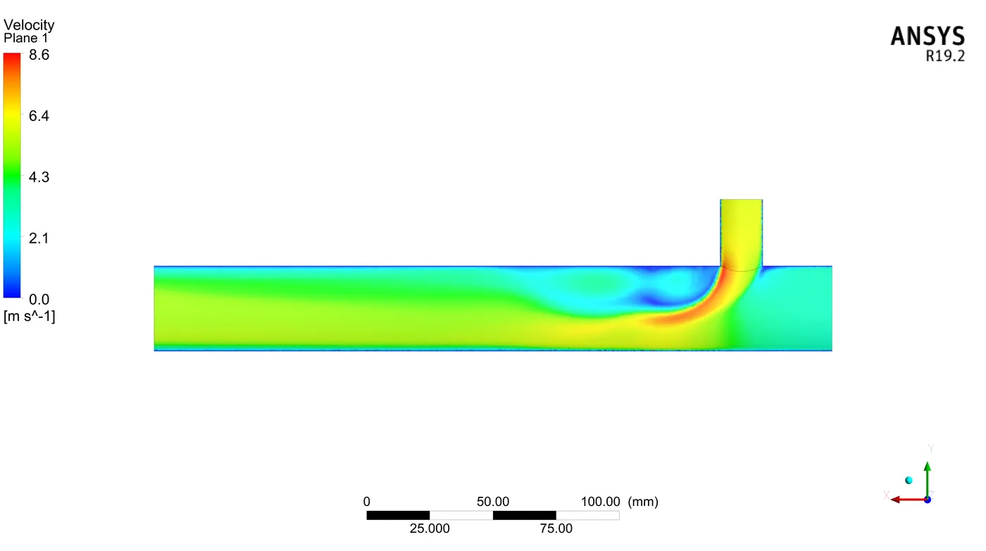
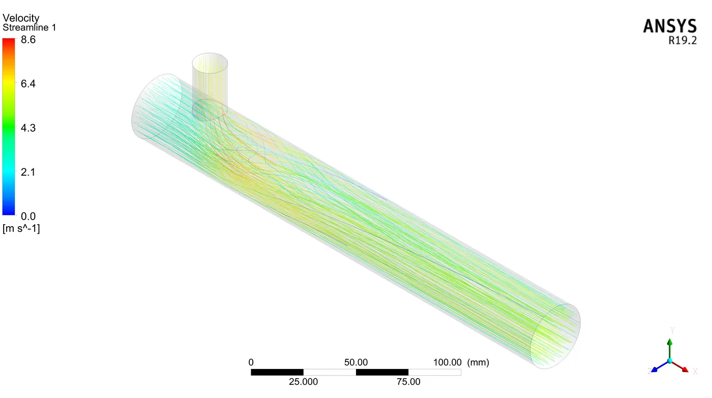
The long pipe with a low momentum ratio as compared to other results doesn't create a special impact. the temp stability is achieved but the mixing of fluid in the k epsilon model is not achieved. In a plane temperature contour, the hot fluid at the lower boundary does not mix properly with cold fluid. The contribution of an increase in the length of the pipe not created very much difference in the result.

• LONG PIPE WITH MOMENTUM RATIO 4 -

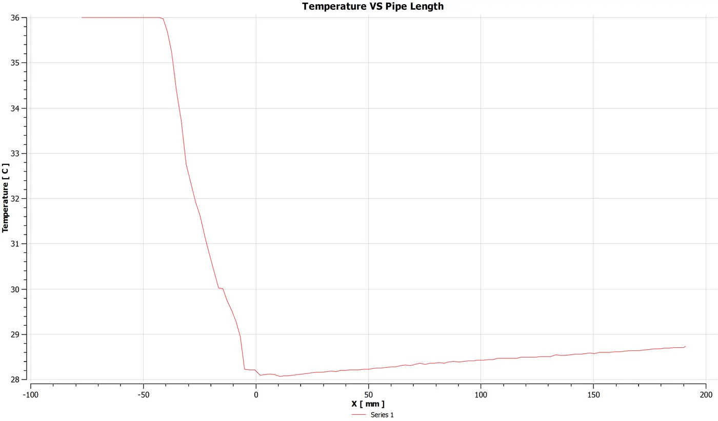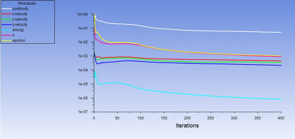
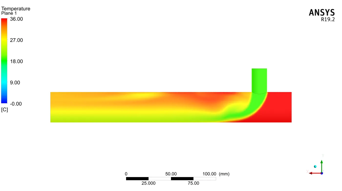
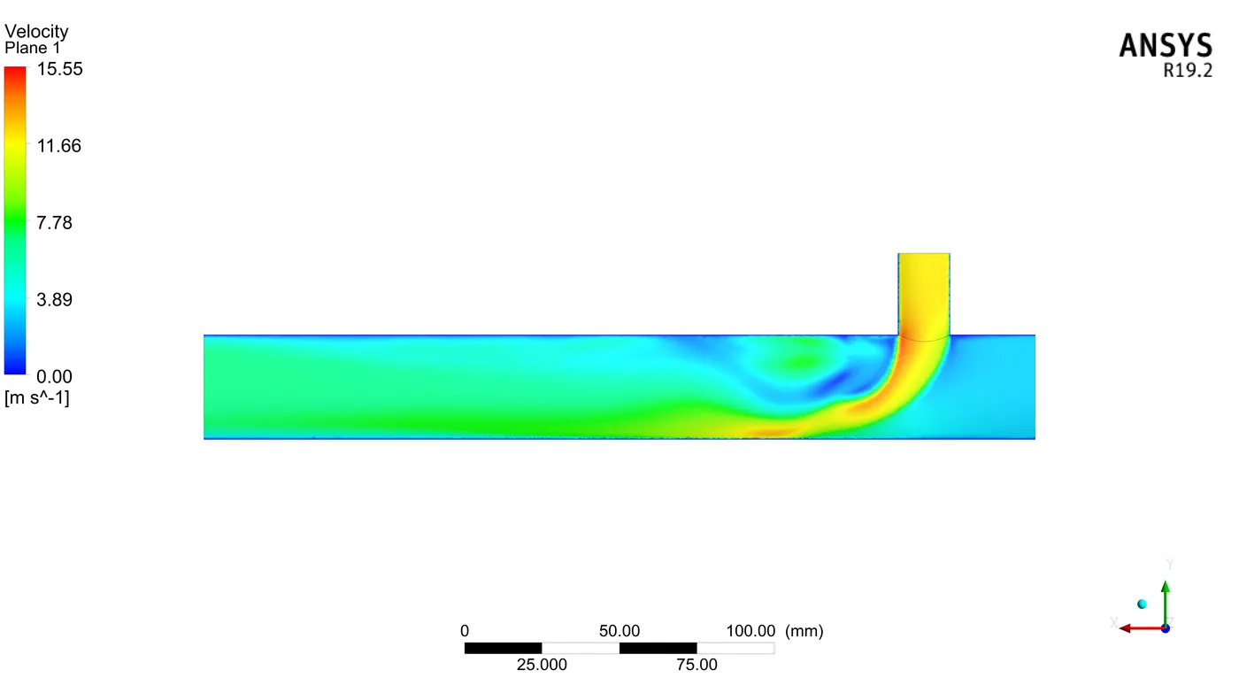
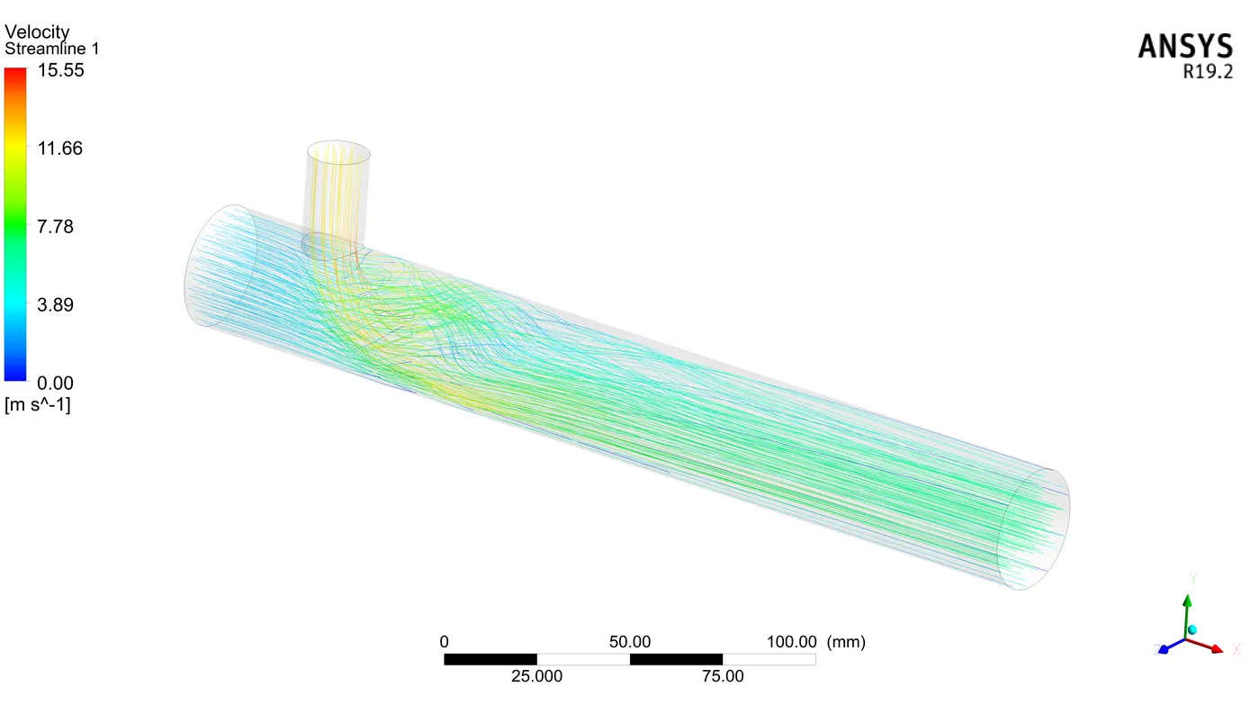
With a long pipe and higher momentum ratio, the mixing of fluid is quite proper at the outlet. The velocity and temperature plane contour results are self-explanatory in this case. The mixing and temperature stability of fluid at the outlet is quite impressive. The momentum ratio effects more as compared to increase in length. The chart shows the proper mixing of the fluid and the temperature variation along the length of the pipe.

From the above study and graphs analysis,

For momentum ratio = 2,

Table 7. Convergence and Temperature at the outlet

Pipe domain	Models	Convergence (Iteration)	Area weighted of Average of temp (C)
Short pipe	K omega SST	262	30.2
Short pipe	Realizable k epsilon	178	30.8
Long pipe	Realizable k epsilon	170	31.4

For momentum ratio =4,

Pipe domain	Models	Convergence (Iteration)	Area weighted of Average of temp (C)
Short pipe	Realizable k epsilon	175	30.9
Long pipe	Realizable k epsilon	229	31.5

An increase in the momentum ratio leads to an increase in the time required for converging the solutions. The number of iterations also increases. But the convergence is the main criterion that has to satisfy in every case.

The temperature at the outlet can be calculated and compared with simulated results by using the following formula :

`Tmix = (m(hot)*T(hot)+m(cold)*T(cold))/(m(hot)+m(cold))=(0.003103*36+0.0016574*19)/(0.0033103+0.0016574)=31.6488C`

• Conclusion -

The study basically focuses on the results by changing the length of the pipe and momentum ratio. The increase in momentum ratio ensures the lowering of temperature at less distance of pipe. The length of the pipe majorly effects on mixing of fluids and stability in temperature at the outlet. The effectiveness of mixing of fluid depends upon enough length to stabilize the result and high momentum ratio to ensure the mixing fast. But as we increase it may result in an increase in an eddy. K epsilon model is used which shows much accurate results as compared to k omega in the above case only.

The above study is carried out in ANSYS Fluent 19.2.