Week 5 - Rayleigh Taylor Instability

AIM:- To Perform the Rayleigh Taylor instability simulation

Objective:-

- To develop the setup for the Rayleigh Taylor instability simulation for 2 different fluids

- To perform the Grid independency test and understand its effect.

- To calculate the Atwood number and understand the effect of the behavior of the instability due to variation in Atwood number.

Theory:-

Introduction - The fluid interface becomes unstable when a heavier fluid is placed over a lighter fluid in a gravitational field. A perturbation of this interface has a tendency to increase with time, producing a phenomenon is known as Rayleigh–Taylor (RT) instability. This phenomenon describes the entrance of the fluid with a higher density into the fluid with lower density in the form of mushroom-shaped protrusions. The RT instability phenomena were initially discovered by Rayleigh and after that applied to the explanation of all accelerated fluids by Taylor. This instability has also been used to describe a wide range of problems, such as inertial confinement fusion, supernova explosions and remnants, nuclear weapon explosions, oceanography, and atmospheric physics, and was for the first time numerically implemented in the 1970s.

Rayleigh-Taylor phenomena-

- The instability of a heavy fluid layer supported by a light one has generally known as Rayleigh-Taylor (RT) instability.

- It can occur under gravity and, equivalently, under an acceleration of the fluid system in the direction toward the denser fluid. A simple example may illustrate typical evolution times for the overturn of ordinary liquids under the effect of the earth's gravity. Assuming an acceleration a = 9.8 m/s

- The first experiments by Lewis have shown three subsequent stages in the evolution of an unstable air-water interface. The initial phase of exponential growth is followed, first, by a transition phase of bubble formation and then by an asymptotic stage of rising air columns.

- In the instability problem, one is mainly concerned with the modification of instability growth rates by various physical effects.

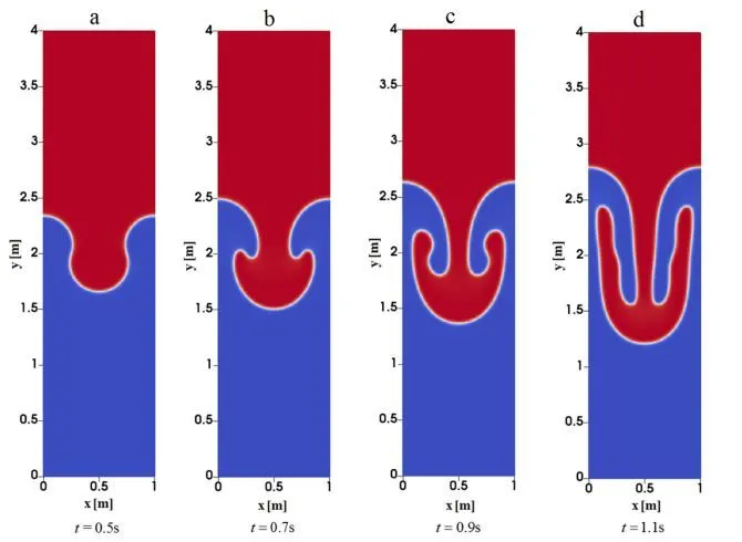
An overview of characteristic flow patterns in the evolution of RT instabilities is given by the schematic drawings of fig.

- The Rayleigh-Taylor instability (RTI) evolves at the unstable interface of two fluids of different densities subjected to a common acceleration normal to the interface. In this situation, small interfacial perturbations evolve into mushroom-like structures with wavelength λ and amplitude a that both increases as time progresses.

- The fluid interchange decreases the potential energy content of the system which is the cause of instability. The further upward motion of the lighter fluid assumes the form of rising gas bubbles with an approximately steady shape.

- These horseshoe-like deformations are based on incompressible inviscid fluid dynamics.

- Typical features of the falling heavy fluid are represented. In a low-density gas, the fluid particles can closely approach the stage of free fall.

- A corresponding contraction of the downward flow gives rise to needle-shaped spikes. When the flow resistance of the lighter fluid becomes important, broadening of the spike tips is observed along with the formation of mushroom-like vortex motions.

- These additional structures are commonly attributed to secondary shear flow instabilities. The pronounced differences between bubbles and spikes disappear for fluids with nearly equal densities. Corresponding bubble-spike pairs can be recognized.

- In the RT instability, the fingers of the lighter fluid penetrate the heavier fluid as bubbles, while the spikes of the heavier fluid move into the lighter fluid.

Atwood number (A)- It is a dimensionless number in fluid dynamics used in the study of hydrodynamic instabilities in density stratified flows. It is a dimensionless density ratio defined as

`A = (rho1 - rho2)/(rho1 + rho2)`

where,

`rho1` = density of the heavier fluid

`rho2`= density of the lighter fluid

In Rayleigh–Taylor instability, the penetration distance of heavy fluid bubbles into the lighter fluid is a function of the acceleration time scale, `A g t^2` where A is Atwood number, g is the gravitational acceleration and t is the time.

In the RT instability, the fingers of the lighter fluid penetrate the heavier fluid as bubbles, while the spikes of the heavier fluid move into the lighter fluid.

CFD models that are based on mathematical analysis of Rayleigh-Taylor waves-

1. Mass diffusion model - The mass diffusion equation describes the transport of mass and energy due to model viscosity and hence drives actual mixing in the fluids. Even if any configuration is Rayleigh-Taylor unstable, the diffusion process could be responsible for significant mixing if the viscosity is sufficiently large.

2. Single fluid model

Potential flow model - This model is valid for all instability changes from the very linear stage through the early non-linear but limited to Atwood number of 1. In this model, the single-mode perturbation expands, the flow equation to second order around the bubble tips, hence obtaining an ordinary differential equation for the bubble velocity.

Buoyancy drag model - It is valid for every Atwood number but limited to non-linear stages of the instability. It uses ordinary differential equations to evolve the width of the mixing layer. The bubble, spikes, or amplitudes are described by balancing the inertia, buoyancy, and drag forces. This model cannot deal with multiple mixing interfaces; cannot be easily extended to two or three dimensions, and as a rule, does not address demixing, also known as counter gradient transport i.e. reduction of total fluid masses within the mixing zone. To address the above problems, two-fluid (multi-fluid) models have to be used.

Besnard-Harlow-Rauenzahn (BHR) - It is a more advanced version of the single-fluid model. The BHR model is based upon the evolution equations arising from second-order correlations and gradient-diffusion approximations. Using a mass weighted-averaged decomposition, the original BHR model includes the full transport equation for Reynold's stresses, turbulent mass-flux velocity, density fluctuations, and turbulent kinetic energy dissipation rate.

3. Multi-fluid models - These models use a separate set of equations for each fluid in addition to the main flow equations and provide an accurate modeling framework for demixing by correctly capturing the relative motion of different fluid fragments.

Two equation K-L turbulence model - The K-L turbulence model involves an equation for turbulent kinetic energy (K) and turbulent length scale (L). The starting point for deriving the model equations is the buoyancy-drag models for the self-similar growth for RT instabilities.

Three equation K-L-a turbulence model - The three equation model was developed as an extension to the two-equation K-L model by including a third equation for the turbulent mass-flux velocity.

Four equation K-L-a-b turbulence model - The four equation model was developed as an extension for the three equation K-L-a model by including a fourth equation for density-specific volume covariance. The model can accurately reflect the effect of changes in the density fluctuations

Cases -

Case 1 - Perform the Grid independence for 0.5mm mesh size and 0.1mm mesh size.

Case 2 - Do the study for different Atwood numbers.

Procedure-

ANSYS Workbench (Fluent) is used for the solution.

Geometry

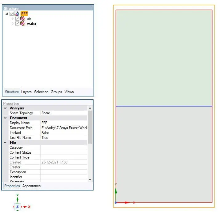
- Geometry is created in SpaceClaim with two different components (surfaces) named air and water.

- Both the component is created with the same surface size of 20mm x 20mm

- In properties share topology is selected so that both surfaces will be interacting with each other and must share information.

CASE - 1 For different Mesh sizes

Mesh Type	Coarse	Refined
Element Size	0.5 mm	0.1 mm
Material	Air and Water	Air and Water
Atwood Number	0.9975	0.9975
Total number of cells	3200	24642

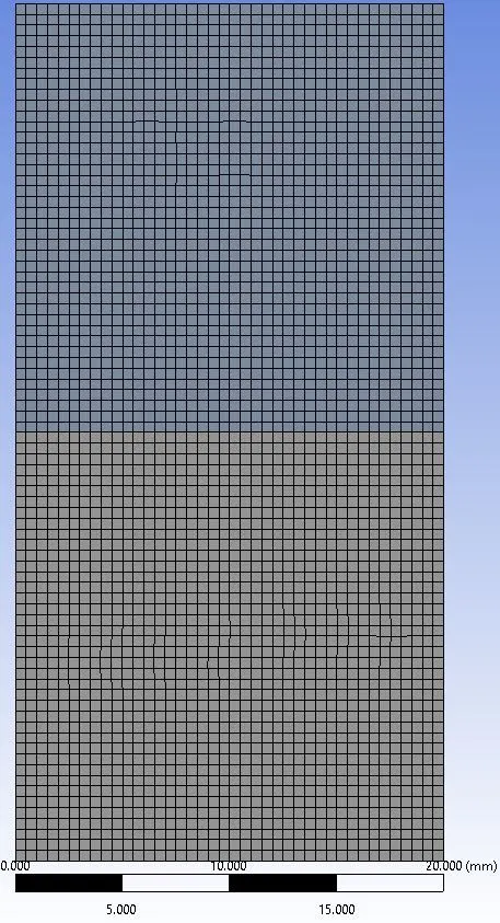
Mesh - A baseline Coarse mesh is created

Coarse mesh - 0.5mm

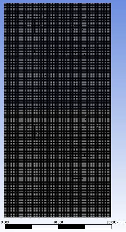
Refined mesh - 0.1mm

Setup 1-

Solver Type	Pressure-Based
Velocity Formulation	Absolute
Time	Transient
Viscous Model	Laminar
Material	Fluid type: Air- 1.225 kg/m3 Water- 998.2 kg/m3
Atwood number	0.9975
Boundaries	Gravity - 9.81 (negative y-direction)

- Before starting simulation Patching of the volume for both phases.

- Water Phase used for patching and volume fraction of "1" is taken for water surface and "0" for air surface

Post - Processing

Coarse mesh - 0.5mm

Refined mesh - 0.1mm

Observation -

- In the first case, baseline (coarse) mesh produced initial results, the results obtained using coarse mesh lack the resolution of the numerical solution. This case initially confirms the setup and is further used for the next case studies. The interface is a bit thicker because of the coarser mesh, which has cell centroids spaced a bit away from the interface. As a function of time advancement, the interface gets smeared out due to numerical diffusion within the interfaces. This causes inappropriate capture of instabilities at the interface.

- The case of finer mesh resulted in good resolution of the numerical solution due to the small/finer interface. This is because more cells capture the volume of fluid and provide fluidity to numerical solutions. Whereas in case 1 numerical solution was comparatively stiff. Furthermore, the instabilities grow exponentially and the simulated results look quite realistic as compared to the results obtained in case 1.

CASE - 2 For Different Atwood Number

Note- For this case, I have taken the mesh size - 0.18, in order to reduce the computational time.

Mesh Type	Refined
Element Size	0.18 mm
Material	User-defined and Water
Atwood Number	0.4278
Total number of cells	24642

Mesh - Refined mesh of 0.18mm

Setup 2-

Solver Type	Pressure-Based
Velocity Formulation	Absolute
Time	Transient
Viscous Model	Laminar
Material	Fluid type: User-Defined- 400 kg/m3 Water- 998.2 kg/m3
Atwood number	0.4278
Boundaries	Gravity - 9.81 (negative y-direction)

- Before starting simulation Patching of the volume for both phases.

- Water Phase used for patching and volume fraction of "1" is taken for water surface and "0" for User-defined surface

Post - Processing

Case 2 - At Atwood number- 0.4278

Refined mesh - 0.18mm

Observation -

- In this study, Analysis for is Rayleigh Taylor instability is done at different Atwood numbers. The larger density ratio results in a stronger force to develop the interface instability.

- For this case at smaller Atwood number, the density disparity between the two sides of the interface is small and the density distribution of the upper and lower layer is nearly symmetrical. The initial density stratification plays a dominant role and the expansion compression effect has little influence.

- The evolution of interface grows slower with a smaller Atwood number.

- Larger Atwood number results in a larger amplitude of perturbation.

Transient-state simulation over Steady-state simulation-The steady-state analysis is done when the study is focused on the final result. But here in this study, the instabilities information is sensitive and time-dependent and is growing exponentially at each time step. Steady-state simulation is capable to capture those instabilities but the results will not be time-accurate. Though Transient state simulation with reduced time-steps can capture these instabilities at each and every time-steps and time-dependent results can be obtained.

Conclusion-

- The simulation of RT instability has been demonstrated. In all simulations, both fluids are considered immiscible and incompressible.

- Transient simulation approach was implemented to study the Rayleigh-Taylor instabilities.

- In the grid dependency test, the interface thickness has a significant impact on numerical diffusion. The interface thickness reduces with mesh refinement and produces better results at less interface thickness.

- It can be seen easily due to change in Atwood number the lighter fluid penetrate the heavier fluid as bubbles, while the spikes of the heavier fluid move into the lighter fluid.

- The variation in Atwood number, has a direct impact on the perturbation amplitude and evolution of interface growth. The implementation of finer mesh and smaller time-steps gave promising visualization of Rayleigh-Taylor instability.

Reference

https://arxiv.org/pdf/2006.12393.pdf

https://sci-hub.yncjkj.com/10.1016/j.enganabound.2017.11.015