Week 5 - Rayleigh Taylor Instability

Aim: To perform Rayleigh Taylor instability simulation for different mesh sizes.

OBJECTIVE

• To Perform the Rayleigh Taylor instability simulation for 2 different mesh sizes with the base mesh being 0.5 mm.
• To compare the results by showing the animations( Attach them from google drive).
• Explaining why a steady-state approach might not be suitable for these types of simulation.
• To find out the Atwood number for both the cases and explaining how the variation in Atwood number in the above two cases affects the behavior of the instability.

INTRODUCTION

• Kelvin-Helmholtz instability:

• Occurs when there are two fluids flowing at different velocities.
• The difference in velocity cause a shear velocity at the intereface of the two layer.
• This induces shear stress on the other fluid layer and if the surface tension is less then results instability along the interface of two fluid.

• Rayleigh-Taylor instability:

• It is an application of hydro-dynamic stability.
• Occurs between two fluids having different densities.
• As the fluids have different densities, they will try yto reduce their combined potential energy.
• If lighter fluid is in top ,then the system is in stable equilibrium condition.
• If heavior fluid is in top ,then heaviour fluid tends to move downward causing the lighter fluid move upward.Thus, disturbance will grow and lead to turbulent flow.

• Richtmyer-Meshkov instability:

• This is inviscid fluid instability with density stratification.
• RMI is a shock induced interfacial instability and this is important in various areas such as supernova explosion, supersonic combustion,non-uniform turbulence etc.

Some practical CFD models based on analysis of Rayleigh-Taylor waves

• Taylor-Analogy Break up Model :

• It considers the unstable RT waves due to the rapid deceleration of the drops.
• It is based on analogy suggested by Taylor , between an oscillating and distorting droplet and spring mass system.
• The restoring force of spring is analogous to surface tension forces.
• The external force on the mass is analogous to gas aerodynamic force.
• Taylor identifies that ,there is not unique critical weber number for breakup.
• The model predicts the state of oscillation and distortion of droplets.
• This model predicts a velocity of the product dops normal to the path of original parent droplet.
• This normal velocity determines an initial spray angle that is in good agreement with measured spray angles.

• Kelvin-Helmholtz Rayleigh-Tayor (KHRT) Break-up Model

• This break up model introduces the competition of the droplet breakup due to KH aerodynamic instability and RT instabilities.
• Whichever model predicting the fastest onset of an instability dominates the breakup process.
• This model is used to model hollow cone sprays and diesel jets.( helps in simplify atomization submodels)

• Buoyancy-Drag model :

• It is a simple model, based on ODE for estimating the growth of turbulent mixing zone at a interference between fluids of different density due to Richtmyer-Meshkov and Rayleigh-Taylor instability.
• It uses ODE to calculate the bubble and spike distances as function of time.

• K-L turbulence model :

• The model describes the dominant eddies in the mixing zone with equation for their characteristic dimension L and energy per unit mass k.
• The equation are based on succesful buoyancy-drag models for RT and RM flows.

SOLVING AND MODELLING APPROACH

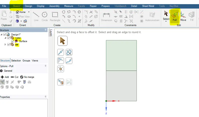
Fig.1 Geometry creation

• In geometry creation , simply sketch a two squares with dimensions 20*20mm and use PULL command to create surface.
• Then create new component as air and water under design section.

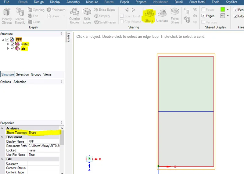
Fig.2 Creating share topology

• Create share topology in order to share the mesh information at the interface of two squares namely air and water(generally two fluids).

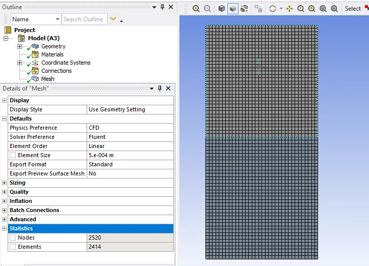
Fig.3 mesh size element 0.5mm

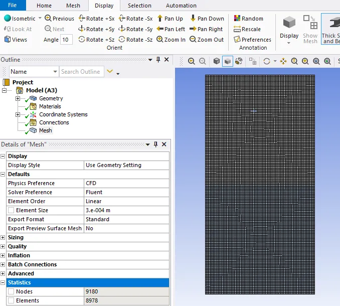
Fig.4 Mesh size element 0.3mm

PRE-PROCESSING AND SOLVER SETTING

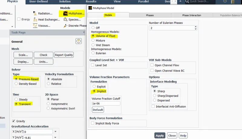
Fig.5 Setting up multiphase models

• We are going to use volume of fluid method which is used to simulate two phase flows .
• Two phase include air and water ,having different density.
• Implicit formulation is being used with pressure based solver.
• Transient analysis is done in order to capture the mixing and instantaneous perturbations.

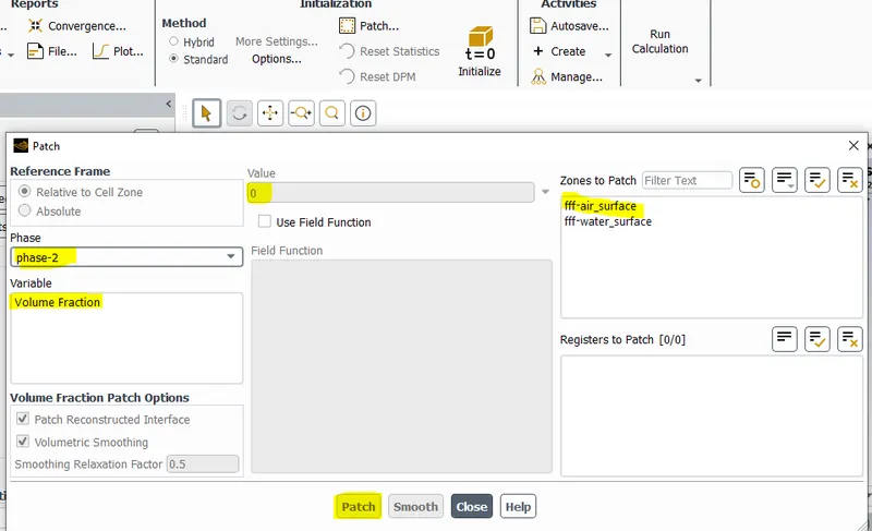
Fig.6 Patch

• Assigning volume fraction to water and air zones respectively by patch .In water phase we have no air phase,so patch it as zero and 1 for water.

RESULTS

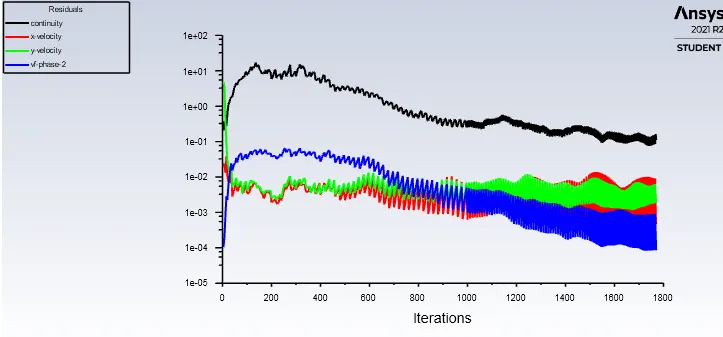
Fig.7 Residual vs iteration 0.5mm

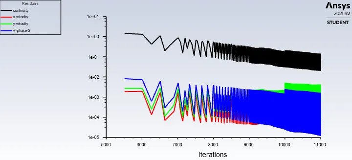
Fig.8 residual vs iteration (0.2 mm )

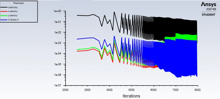
Fig.9 Residual Vs iteration (0.3mm)

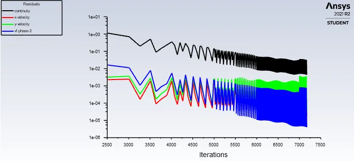
Fig.10 Residual vs iteration (User defined mesh=0.3mm)

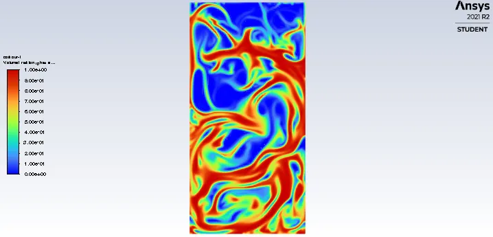
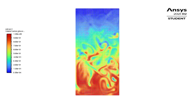
Fig.11 animation at 200 frame (0.2mm mesh size) Fig.12 animation at 200 frame (0.3mm mesh size)

• As we refining the mesh size, the disturbances or instabilities are more precisely captured as it is showing the bubble and spike formation.
• In the base mesh size at 200 animation frame, we observed that steady state is reached, as refining the mesh is taking place the instability perceived for longer duration.

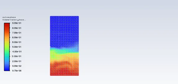
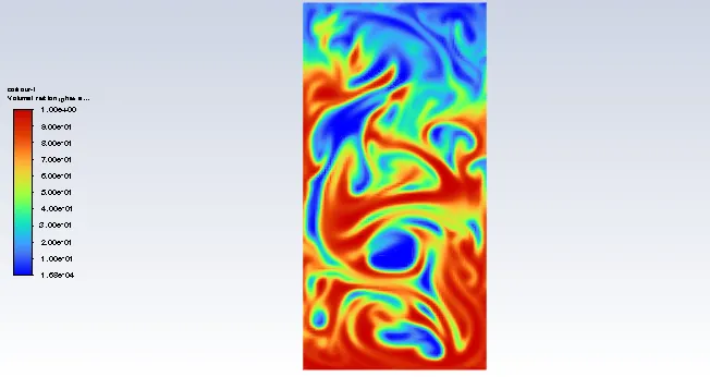
Fig.13 animation at 200 frame ( 0.5mm base mesh size) Fig.14 animation at 200 frame (0.3mm mesh size

User defined fluid

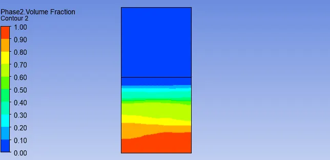
Fig.15 Contour showing volume fraction of water (0.5mm mesh size )

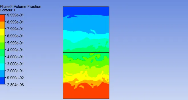
Fig.16 Contour showing volume fraction of water (0.3mm mesh size )

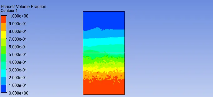
Fig.17 Contour showing volume fraction of water (0.2mm mesh size )

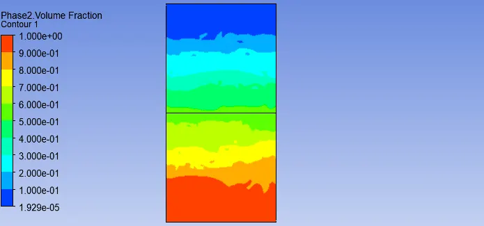
Fig.18 Contour showing volume fraction of water (0.3mm mesh size and user defined)

• Rayleigh taylor base mesh You-tube link
  

https://youtu.be/VERSRxNqIv4

• google drive link base mesh
  

https://drive.google.com/file/d/1pu_IwLwQK77OvFnpdaX_TK1gd-ReXl-4/view?usp=sharing

• Refined mesh 0.3mm You-tube link
  

https://youtu.be/xUMD9lKquNY

• Google Drive link 0.3mm

https://drive.google.com/file/d/1ZpkdghFbnn3l4V4hJYpdl0L5CbyJpkcG/view?usp=sharing

• Refined mesh 0.2mm You-Tube link

https://youtu.be/nYrggqMh9yI

• Google drive link

https://drive.google.com/file/d/1nmeTSh0n4MRPvJHvcx4u11rUCXSaQtMu/view?usp=sharing

• User defined mesh 0.3mm you-tube link

https://youtu.be/hCS_F3AEtIU

• Google drive link

https://drive.google.com/file/d/1OhTcjdMEr_diqIwd_C7lRO83JVk8hbKi/view?usp=sharing

• Atwood Number: Dimensionless number in fluid dynamics used in the study of hydro-dynamic instabilities in density stratified flows.

A = `(rho_1-rho_2)/(rho_1+rho_2)` `rho_1=`Density of heavier fluid

`rho_2 =`Density of lighter fluid

• Atwood number for water and air: `(rho_1-rho_2)/(rho_1+rho_2)`=`(1000-1.225)/(1000+1.225)`=0.997
• Atwood number for water and User-defined fluid: `(rho_1-rho_2)/(rho_1+rho_2)`=`(1000-400)/(1000+400)`=0.428
  

• Atwood number close to 1 signifies that, density difference between the fluid is large.So highly unstable and small perturbation leads to instability.
• Atwood number less than 0.5 signifies that the density difference is small. There is moderately less instability is observed.

• steady state solver is more focussing on end results, so far as disturbances are considered we need to visualize at the begining and instantaneous perturbations (i,e bubble formation).
• We may not get converged solution in explicit approach as courant number plays an important role.

CONCLUSIONS

• In real natural fluid flow, instability is encounterd by two fluids if there is density difference at the interface.
• Also if the velocity of two fluids flowing having different in velocity, we observe instability.
• For capturing the instability ,we refined the mesh size from 0.5mm to 0.2. respectively.The finer grids depicts more mixing and perturbations.