Week 5 - Rayleigh Taylor Instability
OBJECTIVE:-
- Some practical CFD models that have been based on the mathematical analysis of Rayleigh Taylor waves.
- Explain how these mathematical models have been adapted for CFD calculations.
- Perform the Rayleigh Taylor instability simulation for 2 different mesh sizes with the base mesh being 0.5 mm. Compare the results by showing the animations.
- Explain why a steady-state approach might not be suitable for these types of simulation.
- Run one more simulation with water and user-defined material(density = 400 kg/m3, viscosity = 0.001 kg/m-s) for refined mesh.
- Define the Atwood Number. Find out the Atwood number for both the cases and explain how the variation in Atwood number in the above two cases affects the behavior of the instability.
Contents:-
- Concept of Rayleigh Taylor Instability and Its CFD Models.
- Solving and Modeling Approach.
- Simulations of RTI with 3 Cases.
- Concept of Atwood number in RTI.
Concept of Rayleigh Taylor Instability:-
Rayleigh-Taylor instability (RTI) is the interpenetration of materials that occurs whenever a light fluid pushes on a heavy fluid (Rayleigh 1883, Taylor 1950). It is a dynamic process whereby the two fluids seek to reduce their combined potential energy.
Rayleigh–Taylor instability, and it may be modeled by two completely plane-parallel layers of immiscible fluid, the denser fluid on top of the less dense one and both subject to the Earth's gravity. The equilibrium here is unstable to any perturbations or disturbances of the interface: if a parcel of heavier fluid is displaced downward with an equal volume of lighter fluid displaced upwards, the potential energy of the configuration is lower than the initial state. Thus the disturbance will grow and lead to a further release of potential energy, as the denser material moves down under the (effective) gravitational field, and the less dense material is further displaced upwards.
This was the set-up as studied by Lord Rayleigh.The important insight by G. I. Taylor was his realisation that this situation is equivalent to the situation when the fluids are accelerated, with the less dense fluid accelerating into the denser fluid.This occurs deep underwater on the surface of an expanding bubble and in a nuclear explosion.
CFD Models based on the mathematical analysis of Rayleigh Taylor waves:
Smoothed-particle hydrodynamics (SPH):-
Smoothed-particle hydrodynamics (SPH) is a computational method used for simulating the mechanics of continuum media, such as solid mechanics and fluid flows. Smoothed-particle hydrodynamics is being increasingly used to model fluid motion as well. This is due to several benifits over traditional grid-based techniques. The first SPH grauntees conservation of mass without extra computation since the particles themselves represent mass. second, SPH computes pressure from weighted contributions of neighboring particles rather than by solving linear systems of equation.
Finally, unlike grid-based techniques, which must track fluid boundaries, SPH creates a free surface for two-phase interacting fluids directly since the particles repersent the denser fluid and empty space represents the lighter fluid.
SINGLE-FLUID MODEL:-
A typical approach used for the analysis of two-phase flows is a mixture model i.e, the individual fluid phases are assumed to behave as a flowing mixture properties. The applied single fluid model is a five equation model consisting of the mass, momentum and energy equations for a vapour/liquid mixture, and two equations describing the formatin and growth of the liquid phase.
TWO-FLUID MODEL:-
Two-fluid model with interface sharpening is validated with Rayleigh-Taylor instability. Under assumptions of isothermal and incompressible flow of two immiscible fluids, we simulated a system with the fluid of higher density located above the fluid of smaller density in two dimensions. Due to the gravity in the system, the fluid with a higher density moves below the fluid with a smaller density.
The initial condition is not a flat interface between the fluids, but a cosine wave with small amplitude, which develops into a mushroom-like structure. Mushroom-like structure in simulation of Rayleigh-Taylor instability later develops into small droplets as result of numerical dispersion of interface (interface sharpening) or to narrow trails with interface diffusion (no interface sharpening). The results of the two-fluid model with interface sharpening are compared to two-fluid model without interface sharpening and single-fluid-model with/without interface sharpening.
TURBULENCE MODEL:-
Turbulence modeling is the construction and use of a mathematical model to predict the effects of turbulence. Turbulent flows are commonplace in most real life scenarios, including the flow of blood through the cardiovascular system, the airflow over an aircraft wing, the re-entry of space vehicles, besides others. In spite of decades of research, there is no analytical theory to predict the evolution of these turbulent flows. The equations governing turbulent flows can only be solved directly for simple cases of flow. For most real life turbulent flows, CFD simulations use turbulent models to predict the evolution of turbulence. These turbulence models are simplified constitutive equations that predict the statistical evolution of turbulent flows
2. Modelling and Solving Approch:-
Pre-processing :
Step1: Create the Geometry in 2D
We have created a 2D geometry in which 2 Square's of 20mm*20mm in dimension.The top square we assume it is Heavy Fluid Surface i.e, Water and the bottom one is lighter fluid surface i.e, Air. That's why we have given the name respect to its heavy and lighter fluid surface Because We have to simulate the flow on the basis of Rayleigh Taylor Instability. So, we have given the name top sqaure is Water and bottom sqaure is Air.
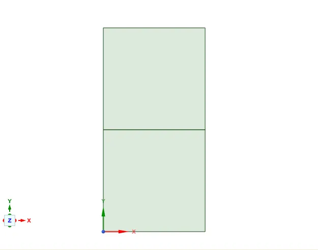
After creating the geometry the common edge between the domains we have to share by sharetopology tool in Workbench. To flow the properties of fluid in one domain to another.
Step2: Meshing
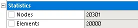
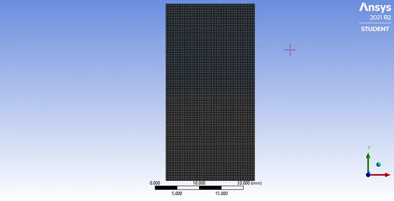
We have created the baseline mesh of element size = 0.5mm. Go to the Mesh properties change the Element size as 0.5mm and right Click on Mesh tool then Click on generate Mesh.

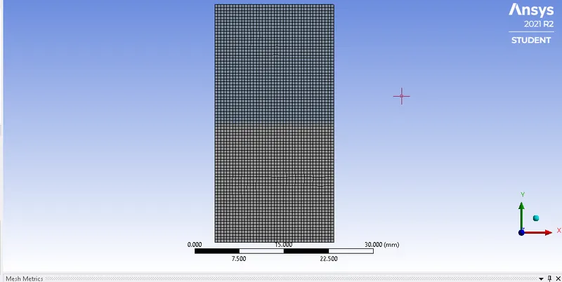
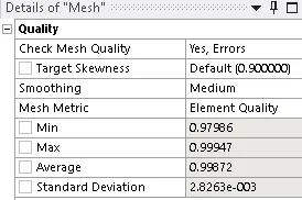
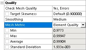
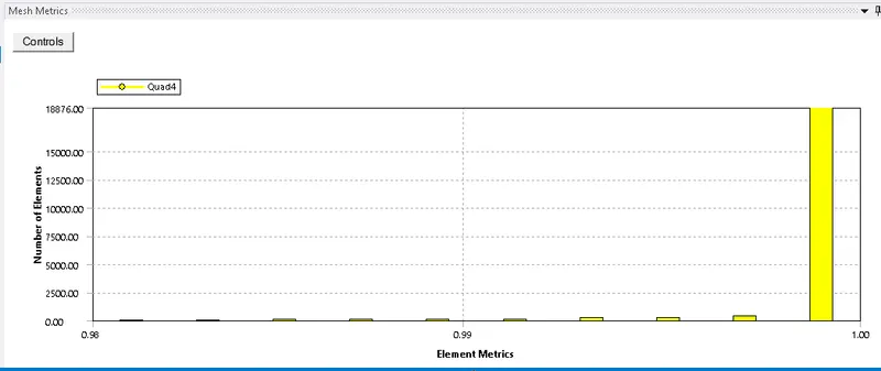
Then Check the Mesh Quality
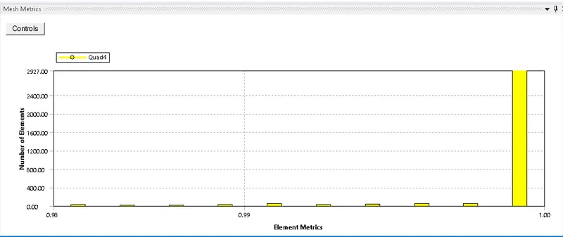
Mesh Steup for Refined Mesh element size = 0.2mm
Step3: Setup Fluent (For Solving)
- Solve - Pressure-based, Transient state solver with Absolute velocity Formulation. Gravity value in negative y Direction = 9.81 m/s^2.
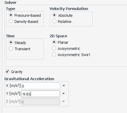
- Viscous Model we have used in the Case is Laminar for low velocity.
- Now, we have to check the Material Properties. In this study we have simulate the 2 cases. In 1st case we have taken two Fluids Water and Air. The Heavy fluid at bottom is Water and the Lighter fluid at bottom is Air.
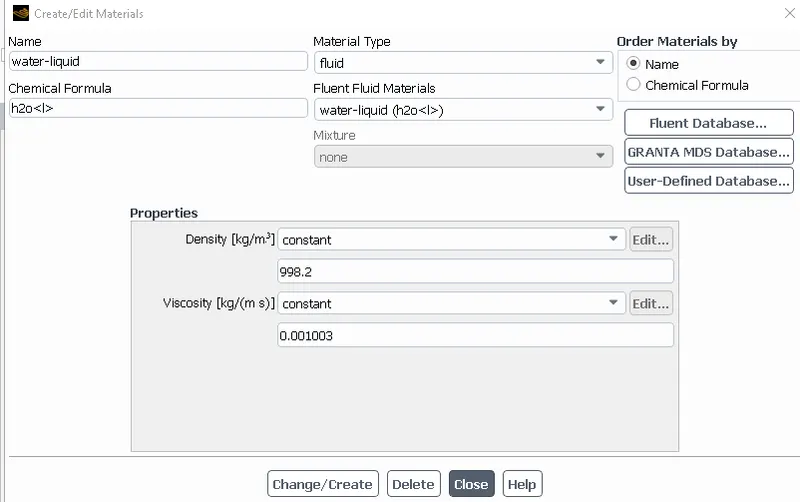
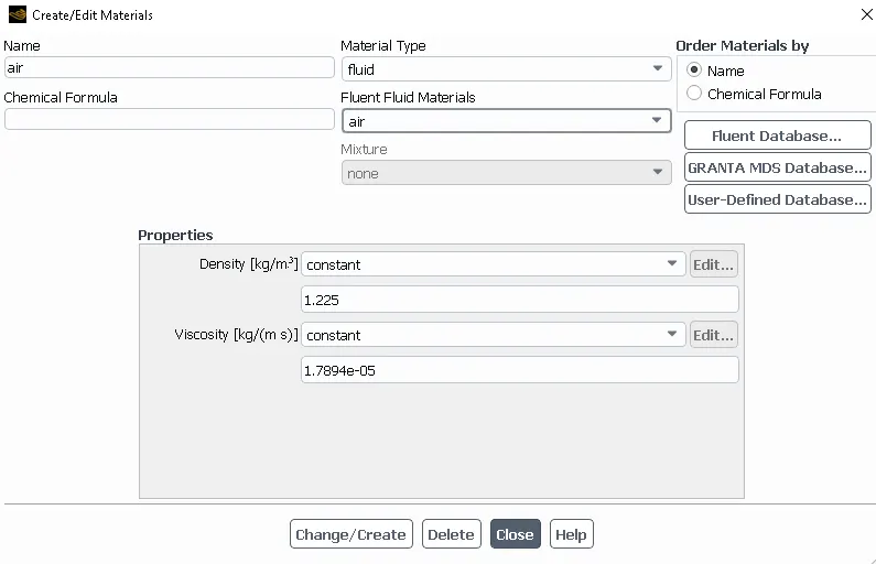
- And For the 2nd case we have taken the Water and Air named as user-defined material with different properties as shown here.
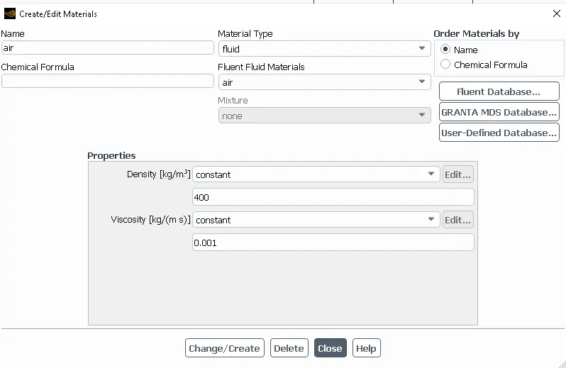
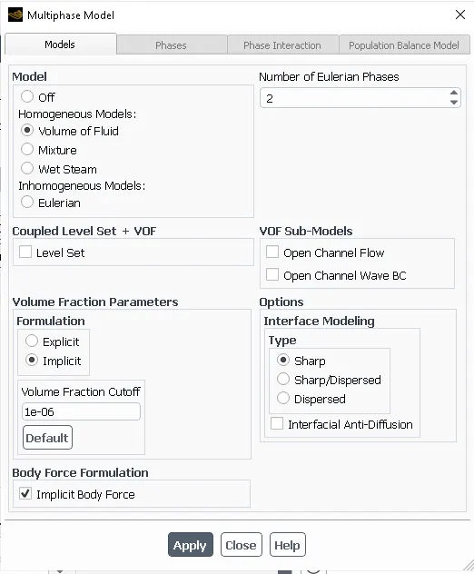
- Multiphase Model - On. It is simultaneous (parallel) flow of materials with different States or phases (Liquid-gas).
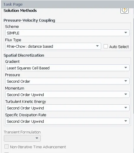
- Solution methods
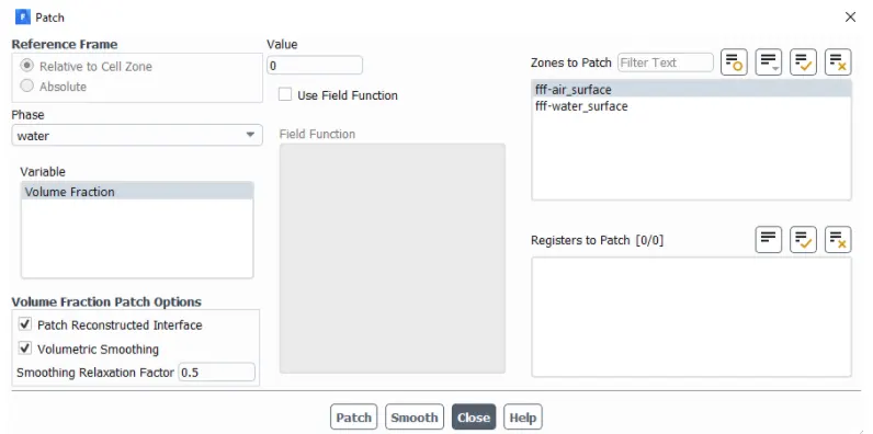
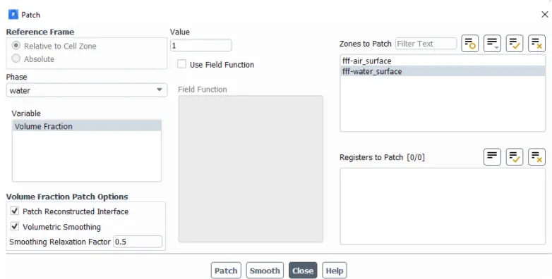
- After the Hybrid Initilalization, We have to Patch the both domains to the respective Heavy and Lighter Fluid. The Heavy Fluid is Water at Top and Lighter Fluid is Air at Bottom. Wheras, we provide the Volume-fraction value of 1 to water and 0 to air.
- After patching we can check the patch has done correct or not by the contours. We setting up for the Contours of Phases - Volume of fluid method at the all surfaces. And After then We go for Calculation. Reduce the Step size as 0.005 and the no. of the time steps we give 1200. and Hit calculate.
Step4: Results
Case1: Baseline mesh element size = 0.5mm (Water and Air)
Case2: Refined mesh element size = 0.2mm (Water and Air)
Case3: Refined mesh element size = 0.2mm (Water and User-defined material)
Conclusion:-
From the above Animations we can observe that Finer Mesh element size 0.2mm Captures the instability better than the coarse mesh element size 0.5mm and As we see the heavier fluid takes more time to settle down as compared to the lighter fluid.
In the Simulation we can clearly see that the state of hydrostatic equilibrium and the RTI is observed at the Interface when the lower density fluid is pushed by the heavy density fluid due to which the formation of the shock waves at the Interface takes place. Formation of air bubbles starts taking place, which compresses the heavy fluid around it, due to which shock waves of multidimensional fashion generates and it gets more stronger as it moves upward.
As we fine the mesh more the simulation results gets more smoother about the irregularities that takes place at the Interface. As higher Density Fluid replaces the lower density air bubbles are formed and also vortex formed, which travels towards the upward region with time.
At the End we can clearly see that two phases gets separated from each other and settle down though we can see diffusivity between them which is a volume fraction of air and water.
Why a steady-state approach might not be suitable for these types of simulation.
As we know In Steady state simulation is preferred to concern more about the final results or the equilibrium state and also you cant see the small-time variation of instability. In RT instability CFD models, we are more concerned to learn about the transition of the irregularities that starts devolping when heavy and low densities fluids mixing under the effect of gravity So, by using the Transient state solver with the refined mesh we can compute the smooth Transition of irregularities takes place at the Interface of the two Fluids.
But the Final state of Steady and Transient State solver must be same and We want to see the behaviour of the solution at every instant of time such that capturing of bubbles, shock-waves, vortex. So, we prefer Transient state solver to see the RT instabilty.
Concept of Atwood number in RTI.
The Atwood number (A) is a dimensionless number in fluid dynamics used in the study of hydrodynamic instabilities in density stratified flows. It is a dimensionless density ratio defined as

where
 = density of heavier fluid
 = density of lighter fluid
Atwood number is an important parameter in the study of Rayleigh–Taylor instability. In Rayleigh–Taylor instability, the penetration distance of heavy fluid bubbles into the light fluid is a function of acceleration time scale, where g is the gravitational acceleration and t is the time.
For Water-Air Instability
density of water () = 998.2 kg/m^3
density of air () = 1.225 kg/m^3
`A = (998.2-1.225)/(998.2+1.225)`
A = 0.998
For Water - User-defined Instability
density of water () = 998.2 kg/m^3
density of Useridefined () = 400 kg/m^3
`A = (998.2-400)/(998.2+400)`
A = 0.428
Variation in Atwood number in the above cases affects the behavior of the instability.
RTI envloves in three disctinct stages: linear stability, bubble Formation, long term evolution due to bubble merging and mixing. When A >0.5 RTI mixing and is shown to recover important statistical measures of the mixing process, such as bubble and spike growth rates and mixing efficiency reported in that study, but at the significantly coarser resolutions typical of most large-eddy simulations. The simulations of RTI at Atwood numbers A>0.9 then used to explore the effects of varying the density ratio on mixing dynamics at very high Atwood numbers 0.75>A>0.95. Spike heights and mixing layer growth rates are shown to be strongly affected by the initial density ratio. An empirical power-law scaling relationship is shown to predict nearly exactly the variation in the ratio of spike to bubble heights as a function of Atwood number.