Week 5: Prandtl Meyer Shock problem

Aim

To simulate a supersonic flow over a convex corner and analyze the Prandtl-Meyer expansion waves. Further, perform a study on the adaptive mesh refinement using various subgrid-scale criteria for temperature and compare the difference in results.

Introduction

Supersonic flows are flows characterized by their flow velocity exceeding the local speed of sound (M>1). This implies that the flow moves fast enough to totally nullify any and all upstream perturbations in the flow. This feature of supersonic flows plays an important role in supersonic flow simulations.

The common boundary conditions used in CFD are:

1. Dirichlet boundary condition
2. Neumann boundary condition
3. Cauchy boundary condition
4. Mixed boundary condition

Out of the above, the Dirichlet and Neumann boundary condition is the most commonly used.

1. Dirichlet Boundary Condition
   This boundary condition applies a specified value for the property at the boundary location. In supersonic flow simulations, this boundary condition type is often used at the inlet to specify static pressure, flow velocity, and temperature.
   
   
2. Neumann Boundary Condition
   This boundary condition specifies a value as the gradient of the property. In supersonic flow simulations, this boundary condition type is often used at the outlet with a value set to zero. This zero gradient outlet implies that all flow properties will be extrapolated from the inlet to the outlet and no information will be transferred in the upstream direction. This boundary condition type is suitable only for supersonic flows since the flow moves fast enough that perturbations in the flow never travel upstream.
   
   

Shockwaves

Shockwaves are strong pressure waves seen in elastic fluids caused by abrupt changes in the motion of supersonic fluids (M>1). Supersonic flows move faster than the speed at which information about oncoming disturbances can propagate upstream, this prevents the flow from being able to react to sudden changes and results in shockwaves. These shockwaves change the properties of the fluid instantly (high temperature and pressure and low velocity and Mach no.) and cause damage to objects in its path. The flow across a shock is always non-isentropic and the strength of the shockwave depends on the angle normal to the flow direction. The strongest shockwave is a normal shock where the shock is perpendicular to the direction of the flow. As the angle decreases, the shock gets weaker and is called an oblique shock. A combination of normal and oblique shockwaves may be seen on blunt bodies and are called bow shockwaves.

Prandtl-Meyer Expansion Fan/Waves

Expansion waves are typically seen in supersonic flows flowing past a convex corner. As the flow turns around the corner, an infinite number of Mach waves emanate from the corner where the flow is seen to gradually turn and accelerate. As the flow accelerates, the pressure, density, and temperature of the flow also decrease. The flow across an expansion fan is gradual and hence is always isentropic. This expansion wave is in many ways the opposite of a shockwave.

Method

Domain and Mesh

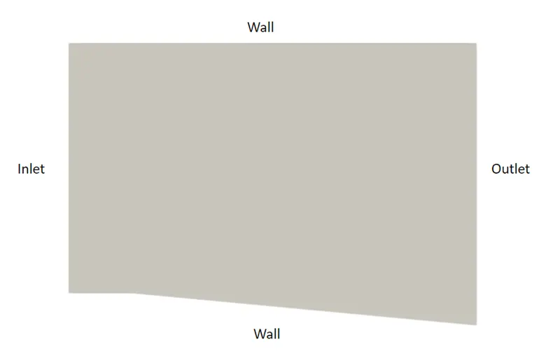
The 2D geometry of the domain was provided and can be seen in the image below.

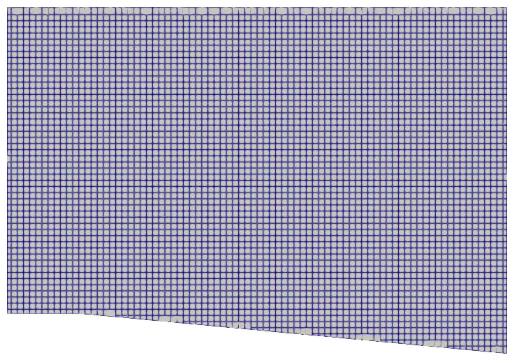
A structured cartesian grid was generated over the geometry using a base sizing of 0.8m. The resulting base mesh contained 4.3k cells as seen below.

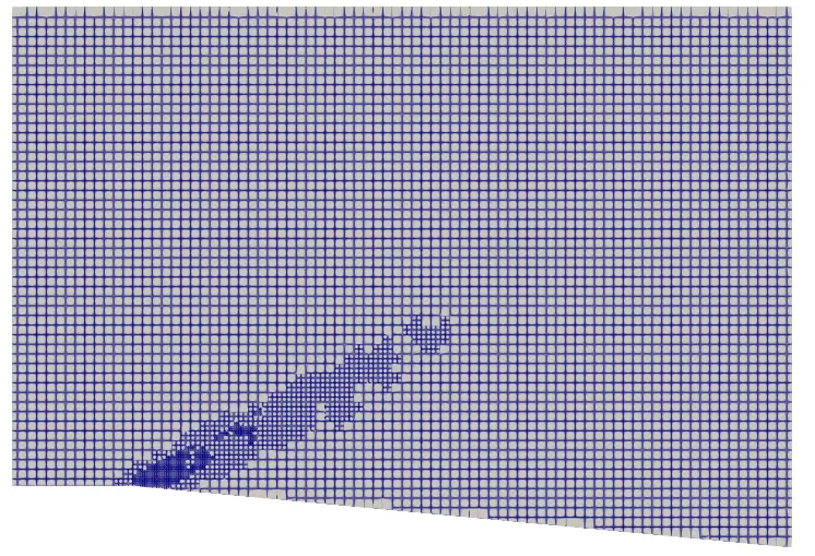
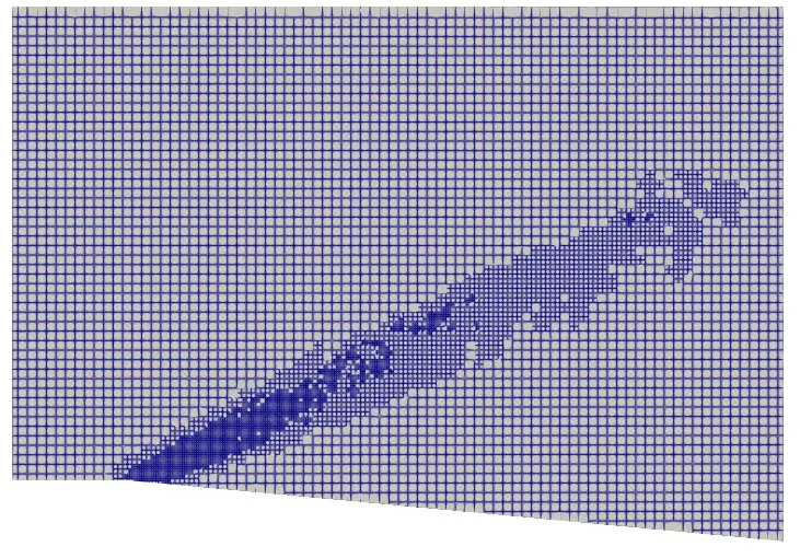
Adaptive mesh refinement was conducted on the base mesh using a scaling factor of 2 and varying subgrid scale criteria for temperature (0.1, 0.05,0.025).

CFD Setup

All Simulations were conducted using Converge v3.0. The fluid used in the domain was air with default properties. Dirichlet boundary conditions were applied for pressure, velocity, and temperature at the inlet while the Neumann boundary conditions were applied at the outlet. At the inlet, the pressure was set to 101000Pa, velocity set to 680m/s, and temperature set to 286K. All the walls in the channel were set to a free-slip condition as the flow is assumed to be inviscid.

The steady-state density-based PISO solver was used for the spatial discretization of the flow parameters. Momentum, density, energy, and species were estimated using the SOR scheme while pressure was estimated using the converge bicgstab scheme. Turbulence in the flow was assumed to be negligible.

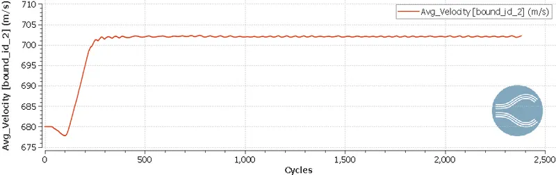
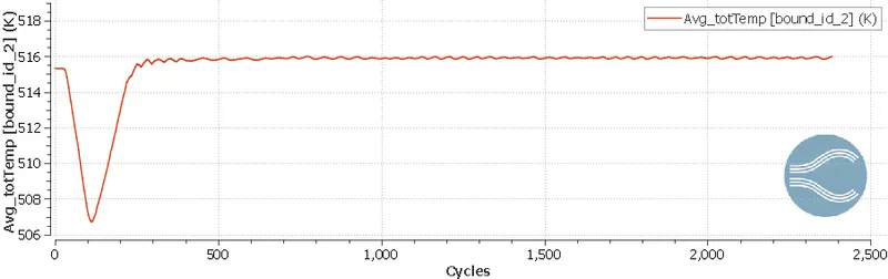
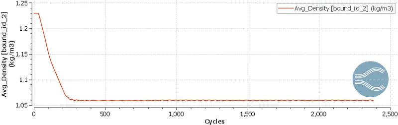
Convergence was monitored using monitors of average velocity, temperature, and density rate at the outlet. The solution was deemed to converge when the monitors varied under 0.001 units across iterations.

Results

The images below show the typical monitors of velocity, temperature, and density at the outlet to ensure convergence for all simulations.

The images below show the final mesh from the adaptive mesh refinement for all simulations.

Case1: SGS Temperature scale = 0.1

Case2: SGS Temperature scale = 0.05

Case3: SGS Temperature scale = 0.025

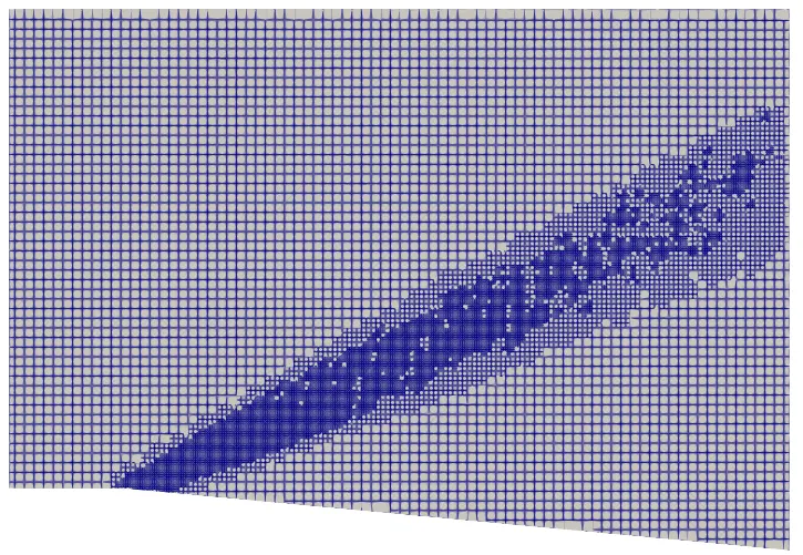
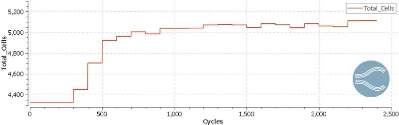
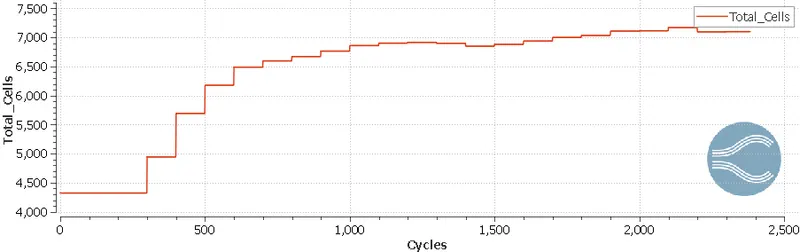
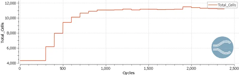
It can be seen that decreasing the SGS scale criterion for temperature creates a denser mesh in the region of the expansion wave. The decrease in scale increases the sensitivity of the solver to detect changes in temperature and thereby creates more refinement. A denser and refined mesh will be able to capture finer details of the flow well but will increase the computational cost of the simulations. Hence, an optimum point between accuracy and computational budget needs to be identified.

The image below shows the variation of the cell count at each iteration.

Case1: SGS Temperature scale = 0.1

Case2: SGS Temperature scale = 0.05

Case3: SGS Temperature scale = 0.025

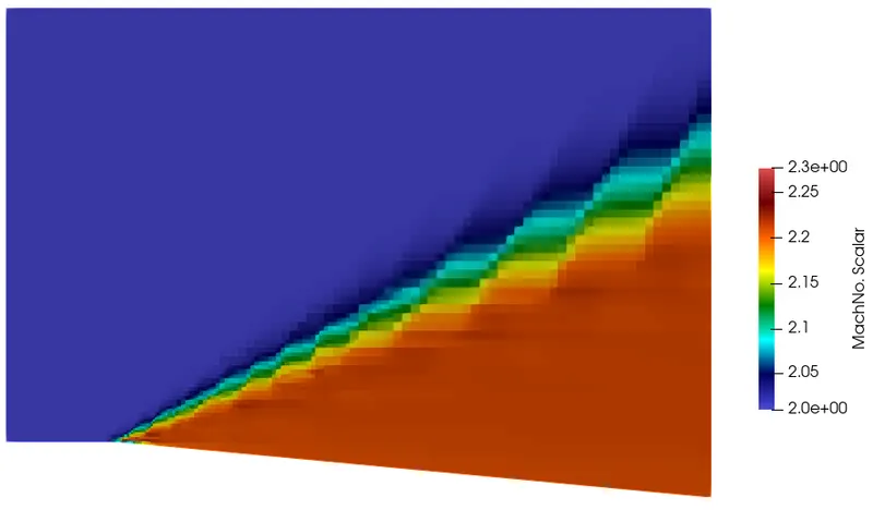
The image below shows the variation of Mach number for all cases.

Case1: SGS Temperature scale = 0.1

Case2: SGS Temperature scale = 0.05

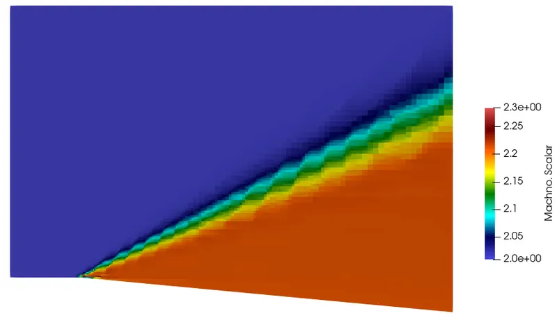
Case3: SGS Temperature scale = 0.025

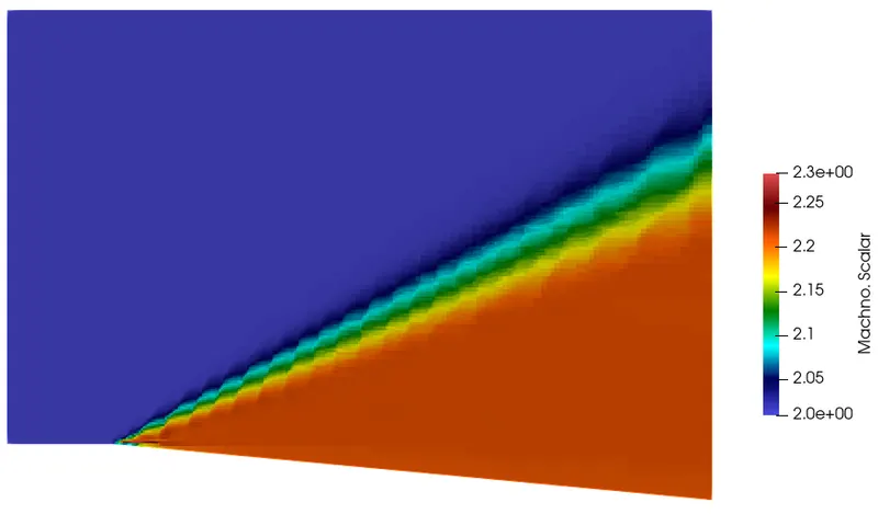
From the images, it is clear that acceleration of the flow occurs at the convex corner. All three cases predict the same increase in Mach no. after the expansion waves. It can also be seen that the increased mesh refinement creates a better resolution of the expansion wave downstream of the corner. The angle and position of the expansion waves are similar in all the cases but only their resolution is varied.

The image below shows the variation of Temperature for all cases.

Case1: SGS Temperature scale = 0.1

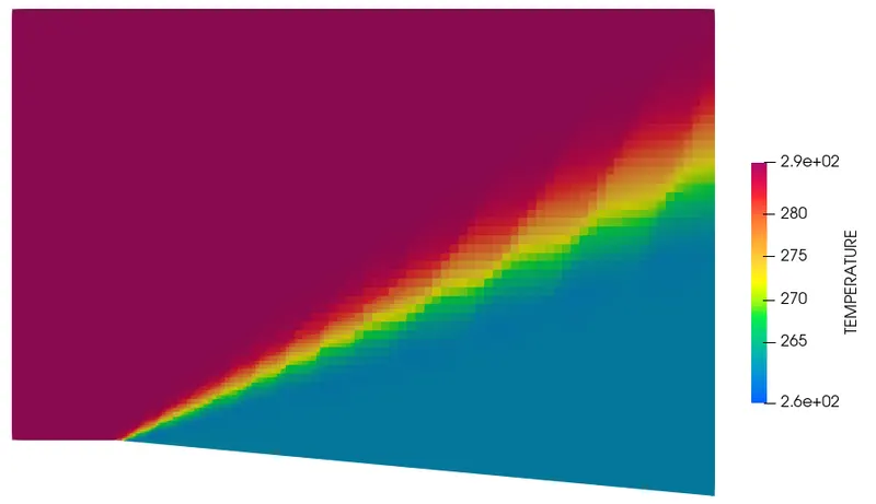
Case2: SGS Temperature scale = 0.05

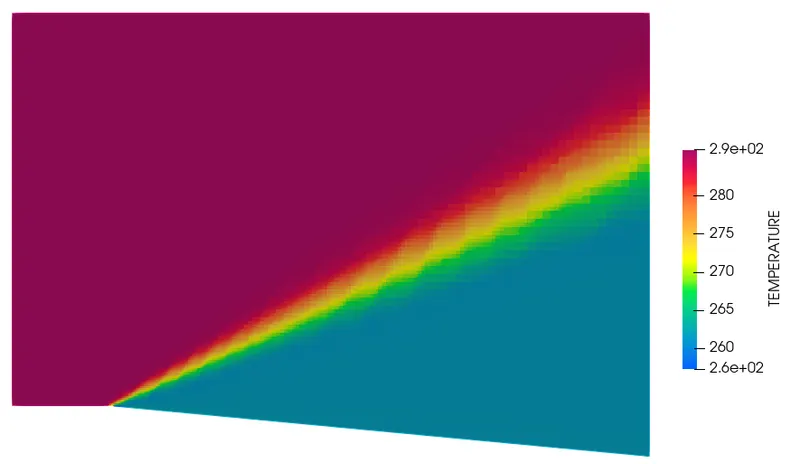
Case3: SGS Temperature scale = 0.025

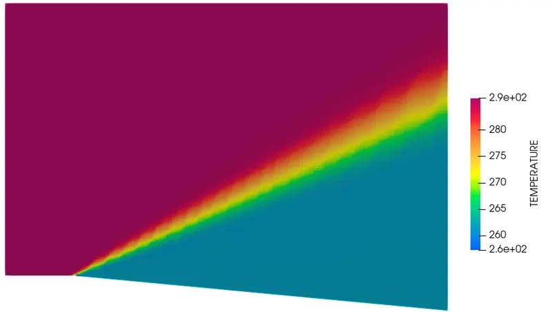
From the images, all three cases predict the same decrease in temperature after the expansion waves. Similar to the Mach no. distrbition, the increased mesh refinement shows better resolution of the expansion wave downstream of the corner. The angle and position of the expansion waves are again similar in all the cases and only their resolution is varied.

Drive link to the animation:

https://drive.google.com/file/d/1f_oCheauG12lxsiBen_a8KUdYm3ypo0O/view?usp=sharing

Conclusion

A supersonic flow over the given convex corner geometry was conducted and the Prandtl-Meyer expansion waves were visualised. Adaptivemesh refinement using varying subgrid scales was conducted and showed increase in total cell count and mesh density in the regions of the expansion wave with decreasing scale factors. The Mach no. of the flow was seen to increase after the expansions waves with a decrease in temperature. The finer mesh was seen to resolve the expansion wave better however the position and anlge of the wave were seen to unaffected by the increased refinements. An optimum value may be identified to ensure desired accuracy of the simulation is achieved without exceeding the computational budget.