Week 5: Prandtl Meyer Shock problem

AIM: Simulating Prandtl Meyer shock problem using converge CFD.

OBJECTIVE:

• To study shock flow boundary condition
• To study physics behind shock waves.
• Effect of sub-grid scale parameter on shock location.

INTRODUCTION:

Prandtl meyer expansion wave

• when a supersonic flow encounters a convex corner, it forms an expansion fan,which consists of an infinite number of expansion waves centered at the corner.
• The leading edge of expansion fan makes an angle `mu_1`with respect to the upstream flow direction and the trailing edge of the wave makes an angle `mu_2`with respect to downstream flow direction.
• The angles `mu_1 and mu_2` are mach angles defined by

`mu_1=arcsin(1/M_1)` `mu_2=arcsin(1/M_2)`

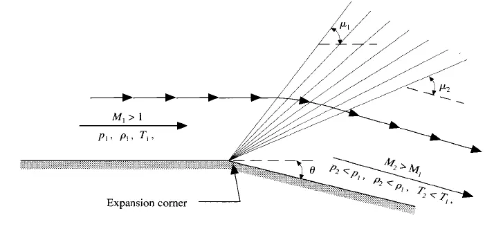
Fig.1 Prandtl meyer expansion wave( John Andersion)

• as the flow passes through the expansion wave,the mach no. increases and the pressure,temp. and density decreases.
• The flow behind the expansion wave is also uniform at mach no. `M_2` and parallel to wall behind the wave.
• The corner point (at which the flow is turned around) is a singular point at which the streamline at the wall experiences a discontinuous change in direction and the flow properties are also discontinuous.
• The flow at the upstream boundary is at mach no. 2,with pressure,temp., density are:

T= 286 K, `rho=1.23 kg/m^3`, P=1 bar

• let 'f' is the Prandtl Meyer function and `theta`is the flow deflection angle then,

`f=sqrt((gamma+1)/(gamma-1))arctansqrt(((gamma-1)/(gamma+1))(M^2-1))-arctansqrt(M^2-1)`

and `f_2=f_1+theta`

• Once `M_2`is obtained,then the prssure,temperature,and density behind the wave are calculated from the isentropic flow relation:

`T_2/T_1=([1+(gamma-1)/2]*M_1^2)/([1+(gamma-1)/2]*M_2^2`

`P_2/P_1=[(1+((gamma-1)/2)*M_1^2)/((1+((gamma-1)/2))*M_2^2]]^(gamma/(gamma-1)`

BOUNDARY CONDITION

There are two boundary condition that the flow has to satisfy :

1. Velocity Boundary condition: Which states that the component of flow velocity normal to the wall be zero.
2. Pressure condition: Which states that there can not be a discontinuity in the static pressure inside the flow.

• Generally a pressure condition can not be used at a boundary where velocities are specified because velocities are influenced by pressure gradient.
• Zero normal gradient boundary condition simply extrapolates the quantity to the patch from the nearest cell value.
• The quantity is developed in space and its gradient is equal to zero in direction perpendicular to the boundary.

• For supersonic flows as the input condition is velocity equal to 680 m/s and pressure inlet is atmospheric so at outlet the velocity is somewhere developed to its final value just at interior to outlet(grid point near to outlet present in interior domain). So, Neumann boundary condition is preferred.

CASE SET UP

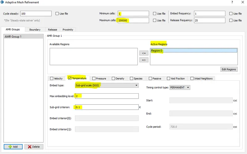
Fig.1 adaptive mesh refinement set up

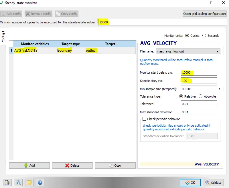
Fig.2 steady state monitor

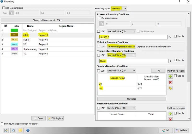
Fig.3 Boundary condition given to inlet

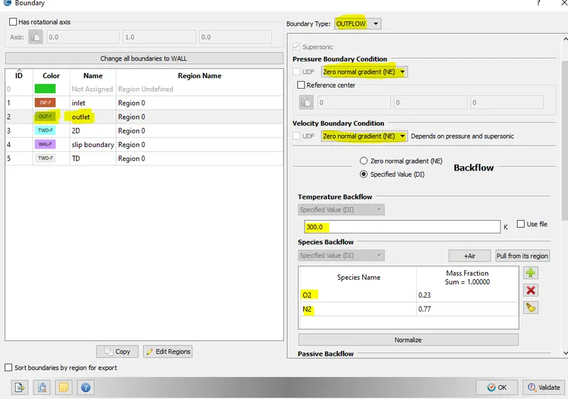
Fig.4 Boundary condition given to outlet

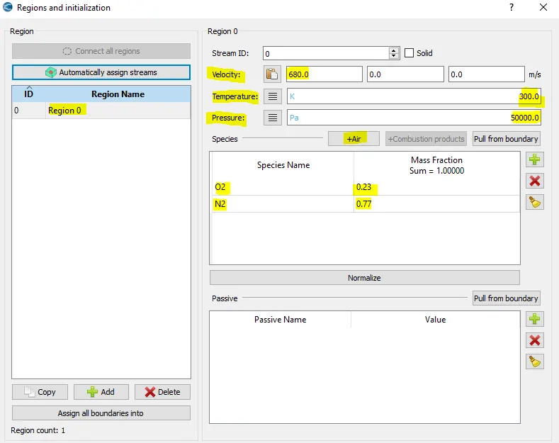
Fig.5 regions and initialization

RESULTS:

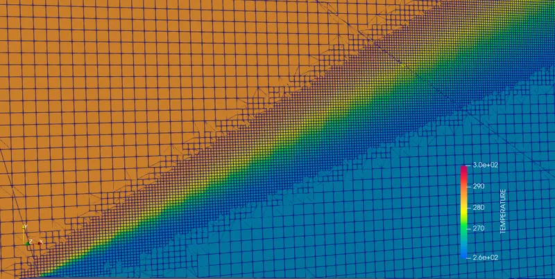
Fig.6 Temperature contour with sgs 0.01

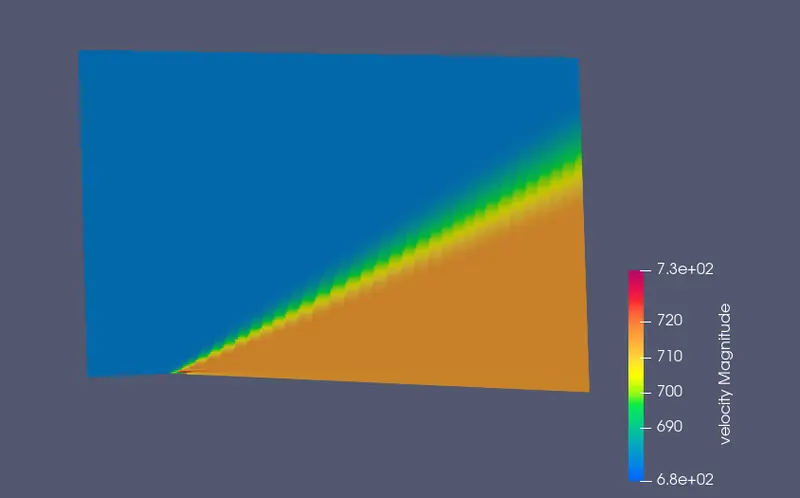
Fig.7 Velocity contour with sgs 0.01

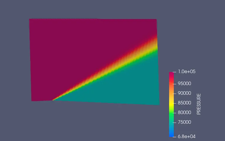
Fig.8 pressure contour with sgs 0.01

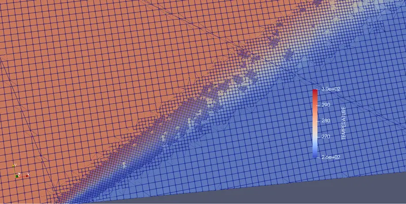
Fig.9 Temperature contour with sgs 0.05

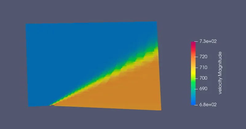
Fig.10 Temperature contour with sgs 0.05

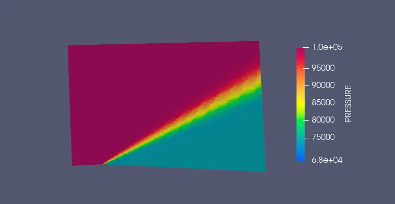
Fig.11 Pressure contour with sgs 0.05

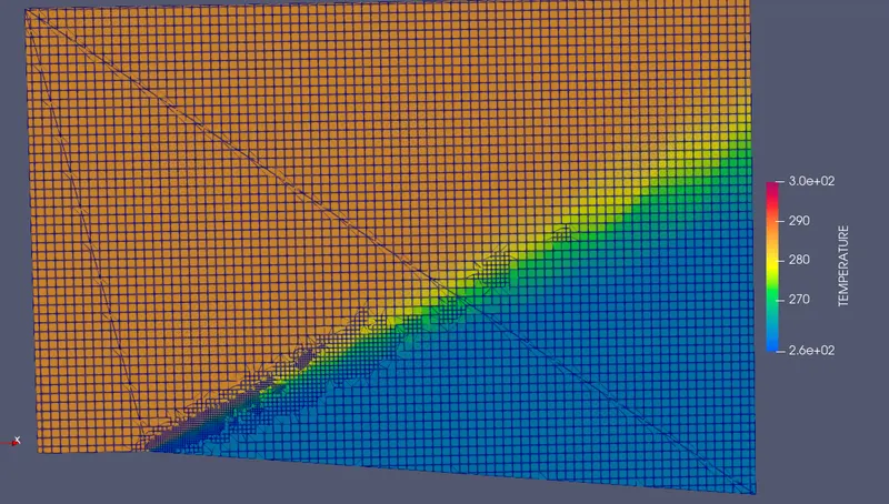
Fig.12 Temperature contour with sgs 0.1 temp

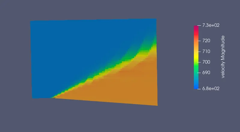
Fig.13 velocity contour with sgs 0.1

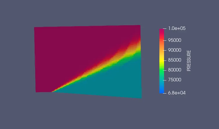
Fig.14 pressure contour with sgs 0.1

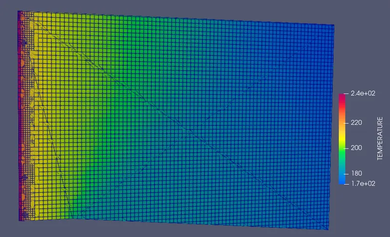
Fig. Tempeature contour for subsonic velocity at inlet .

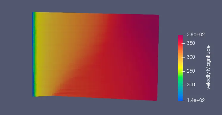
Fig. Velocity contour for subsonic velocity at inlet .

PLOTS

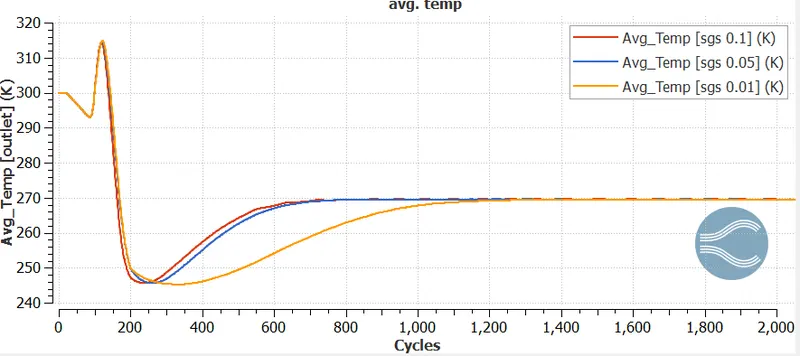
Fig.15 Avg. temperature plot

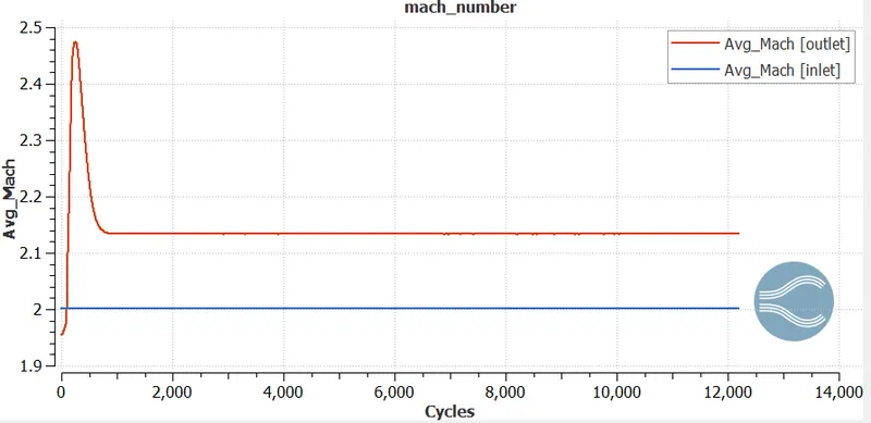
Fig.16 Mcah number

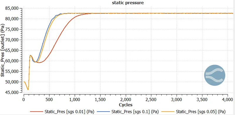
Fig.17 static pressure plot

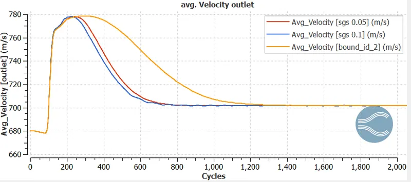
Fig.18

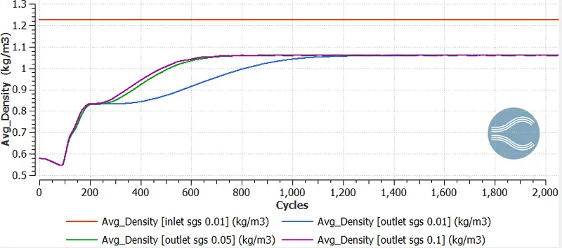
Fig.19

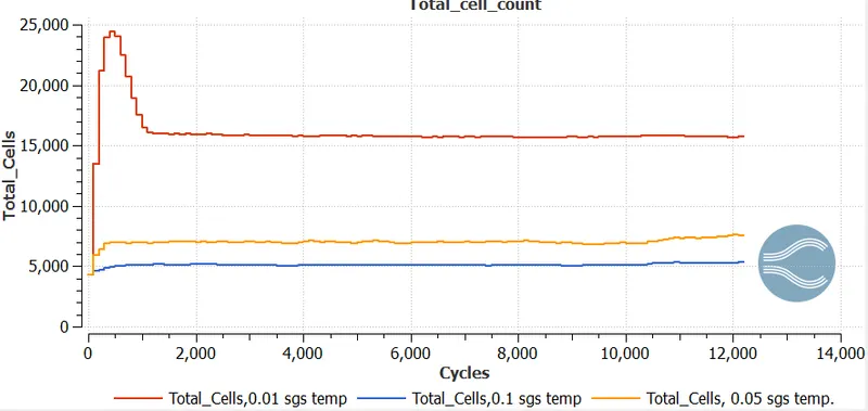
• sub-grid scale of 0.01 , temperature contour animation

https://youtu.be/p_DdHx2r6C8

• sub-grid scale of 0.1 , temperature contour animation

https://youtu.be/sPjt3_7h7mI

• sub-grid scale of 0.05, temperature contour animation.

https://youtu.be/6GXuZzeyS2o

VALIDATION

• To validate the above results we need to find out the percentage error by compiring the numerical and analytical results .
• The anaytical results can be obtained by applying the formula as mwntioned below by taking the fluid as calorically gas and also considering the expansion region undergoing isentropic process.

`f=sqrt((gamma+1)/(gamma-1))arctansqrt(((gamma-1)/(gamma+1))(M^2-1))-arctansqrt(M^2-1)`

and `f_2=f_1+theta`

• By referring the table in John Andersion we get the value for `f(2)=26.37 deg`

so, `theta=f(M_2)-f(M_1)` and `f(M_2)=theta +f(M_1)` we get the value for `M_2= 2.20`

For finding out the temp.,pressure and density use the formula:

`P_2=P_1*[[(1+(gamma-1)/2)*M_1^2]/[(1+(gamma-1)/2)*M_2^2]]^(gamma/(gamma-1))`

`T_2=T_1*[(1+(gamma-1)/2)*M_1^2]/[(1+(gamma-1)/2)*M_2^`

Given the initial condition : T= 286 K, `rho=1.23 kg/m^3`, P=1 bar ,M=1 at subscript 1

so at outlet we are getting the temp., press., and density values as analytical value are : `T_2=261.5 k` , `P_2=0.729`bar

and `rho_2=1.124 (kg)/(m^3)`

Simulation results

`T_2'=269.53k` `P_2'=0.82`bar `rho_2'=1.059`

percentage error : for temperature `(269.53-261.5)/(261.5)`*100 = 0.030*100 = 3 %

similarly for density =6 % and pressure= 3%

CONCLUSION:

• In this project we have studied both cases i.e, supersonic and subsonic flow condition .
• In subsonic flow, the expansion wave corner point is slightly shifted to backward and the wave is not that much prominent as veocity is low.
• For a supersonic flow, the Mach no. increses in wave region whereas all other parameters decreases respectively.
• The effect of sgs temperature on cell count increases as sgs temperature having lower value than higher value.For sgs 0.01 we are having more adaptive mesh refinement cell.