Week 5 - Mid term project - Solving the steady and unsteady 2D heat conduction problem
Aim:
To Solve the 2D heat conduction equation by using the point iterative techniques for Steady state & Transient State heat conduction and write the code for both Explicit method & Implicit method.
Given data:
The Boundary conditions for the problem are as follows;
Top Boundary = 600 K
Bottom Boundary = 900 K
Left Boundary = 400 K
Right Boundary = 800 K
Implementing the following methods for solving implicit equations.
1. Jacobi
2. Gauss-seidel
3. Successive over-relaxation
Your absolute error criteria is 1e-4
Steady state heat conduction:
Steady state conduction is the form of conduction that happens when the temperature differences driving the conduction are constsnt, so that after an equilibrium time, the spatial distribution of temperature in conducting object does not change any further.
General equation for the steady state 2D heat conduction is `(del^2T)/(delx^2) +(del^2T)/(dely^2) =0`
Where `T = Temperature (K)`
`x,y` are space coordinates
`therefore (delT)/(del t) = 0`
Steady state conduction is time independent different equation. Hence both implicit and explicit ,ethods are not applicable.
Final equation for the steady state 2D heat conduction is `T_P = (1/k)*[(T_L+T_R)/(Delta x^2)]+ (1/k)*[(T_T+T_B)/(Delta y^2)]`
Applying the nodes (i,j) in the above equation
`implies``T_(i,j) = (1/k)*[(T_(i-1,j)+T_(i+1,1))/(Delta x^2)]+ (1/k)*[(T_(i,j-1)+T_(i,j+1))/(Delta y^2)]`
Iterative methods:
Iterative method is a mathematical procedure that uses as initial guess to generate a sequence of improving approximate solutions for a class of problems, in which the n-th order approximation is derived from the prevoius ones.
Jacobi method:
Jacobi method is a iterative method at where all updated values are used for the computations only after all the variables have been updated.
Applying the nodes (i,j) in the steady state 2D heat conduction equation
`implies``T_(i,j) = (1/k)*[(Told_(i-1,j)+Told_(i+1,1))/(Delta x^2)]+ (1/k)*[(Told_(i,j-1)+Told_(i,j+1))/(Delta y^2)]`
Gauss Seideil method:
Gauss Seideil method is a iterative method, where the updated variables are used in the computations as soon as they are updated.
Applying the nodes (i,j) in the steady state 2D heat conduction equation
`implies``T_(i,j) = (1/k)*[(Told_(i-1,j)+T_(i+1,1))/(Delta x^2)]+ (1/k)*[(Told_(i,j-1)+T_(i,j+1))/(Delta y^2)]`
Successive Over-Relaxation (SOR) method:
SOR is a variant of the Gauss-Seidel method for solving a system of linear equations, resulting in faster convergence. It is also used for slowly convergence iterative process.
if relaxation factor is <1 then the method is under-relaxed.
if relaxation factor is >1 then the method is over-relaxed.
Applying the nodes (i,j) in the steady state 2D heat conduction equation
`implies``T_(i,j) =(1-omega)*Told_(i,j) +omega* (1/k)*[(T_(i-1,j)+Told_(i+1,1))/(Delta x^2)]+ (1/k)*[(T_(i,j-1)+Told_(i,j+1))/(Delta y^2)]`
MATLAB code for Steady state heat conduction:
%  Steady state analysis
clear all
close all
clc

% Defining inputs
nx=10; % No. of grid points along x axis
ny=10; % No. of grid points along y axis
% Define Mesh
x = linspace(0,1,nx);
y = linspace(0,1,ny);
% Mesh size
dx = x(2)-x(1);
dy = y(2)-y(1);
T=300*ones(nx, ny); % Initializing Temp.
% Applying boundry conditions
T(1,:)=600;     % Top Boundary
T(ny,:)=900; % Bottom Boundary
T(:,1)=400;   % Left Boundary
T(:,nx)=800; % Right Boundary

% Creating a copy
Told = T;
Tinitial = T;
tol = 1e-4; % Tolerence
error_Jacobi = 10;

% Jacobi Method

tic
jacobi_iter = 0;
% Convergence loop
while(error_Jacobi>tol)
        % Space loop
        for i= 2:nx-1
           for j= 2:ny-1
               k = 2*(dx^2+dy^2)/(dx^2*dy^2);
               term1 = (1/k)*(Told(i-1,j)+Told(i+1,j))/(dx^2);
               term2 = (1/k)*(Told(i,j-1)+Told(i,j+1))/(dy^2);
               T(i,j) = (term1+term2); % Jacobi iteration
           end
        end
        error_Jacobi= max(max(abs(Told-T)));
        Told=T; % Updating Told value
        jacobi_iter = jacobi_iter+1;
end
toc
 % Plotting
 figure(1)
 contourf(x,y,T)
 clabel(contourf(x,y,T));
 colorbar
 colormap(jet)
 xlabel('X-axis')
 ylabel('Y-axis')
 title_text = sprintf('Jacobi-Iteration number = %d',jacobi_iter);
 title(title_text)
 set(gca,'YDIR','reverse')


 %  %Gauss Seidel Method

tic
 T = Tinitial;
 Told = Tinitial;
 error_GS = 10;
%Convergence loop
gs_iter = 0;
while(error_GS>tol)
        % Space loop
        for i= 2:nx-1
           for j= 2:ny-1
               k = 2*(dx^2+dy^2)/(dx^2*dy^2);
               term1 = (T(i-1,j)+Told(i+1,j))/(dx^2);
               term2 = (T(i,j-1)+Told(i,j+1))/(dy^2);
               T(i,j) = (1/k)*(term1+term2); %  Gauss seidel iteration
           end
        end
        error_GS= max(max(abs(Told-T)));
        Told=T; % Updating Told value
        gs_iter = gs_iter+1;
end
toc
 % Plotting
 figure(2)
 contourf(x,y,T)
 clabel(contourf(x,y,T));
 colorbar
 colormap(jet)
 xlabel('X-axis')
 ylabel('Y-axis')
 title_text = sprintf('GS-Iteration number = %d',gs_iter);
 title(title_text)
 set(gca,'YDIR','reverse')


 % SOR Method

 tic
 error_SOR = 10;
 T = Tinitial;
 Told = Tinitial;
 w = 1.2;
 error = 1;
SOR_iter = 0;
while(error_SOR>tol)
        % Space loop
        for i= 2:nx-1
           for j= 2:ny-1
               k = 2*(dx^2+dy^2)/(dx^2*dy^2);
               term1 = (T(i-1,j)+Told(i+1,j))/(dx^2);
               term2 = (T(i,j-1)+Told(i,j+1))/(dy^2);
               T(i,j) = (1-w)*Told(i,j)+(w*(1/k)*(term1+term2)); % SOR iteration
           end
        end

           error_SOR = max(max(abs(Told-T)));
           Told = T; % Updating Told value
        SOR_iter = SOR_iter+1;
end
toc

 % Plotting
 figure(3)
 contourf(x,y,T)
 clabel(contourf(x,y,T));
 colorbar
 colormap(jet)
 xlabel('X-axis')
 ylabel('Y-axis')
 title_text = sprintf('SOR-Iteration number = %d',SOR_iter);
 title(title_text)
 set(gca,'YDIR','reverse')
Procedure:
- Initially defined the no.of grid point along x and y axis.
- Next, define the mesh and mesh size.
- Next, apply the initial and boundry conditions (Temperature).
- Next, create the copy of the Initialized temperature.
- Next, define error and tolerance value.
- Next, create the iteration method for jacobi, GS & SOR.
Iteration method:
It consists of two loops,
- Convergence loop
- Space loop
Space loop consists of two for loops to calculate the 'T' value along with the grid points. Since it is of 2D heat conduction equation, two indicies (i & j) are used along x and y axis respectively.
Space loop is inside the convergence loop. convergence loop/While loop is used to control the error value. This while loop will continues untill the error value is greater than tolerance value.
Based on iteration method the 2D equation of 'T' will vary.
After for loop error value is calculated and updateTold as 'T' value.
Next, update the iteration number.
Simulation Results:
- Contours of Jacobi, Gauss seidel and SOR iterations:
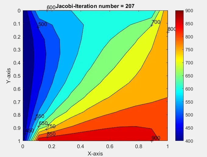
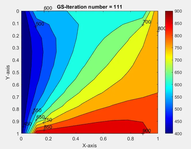
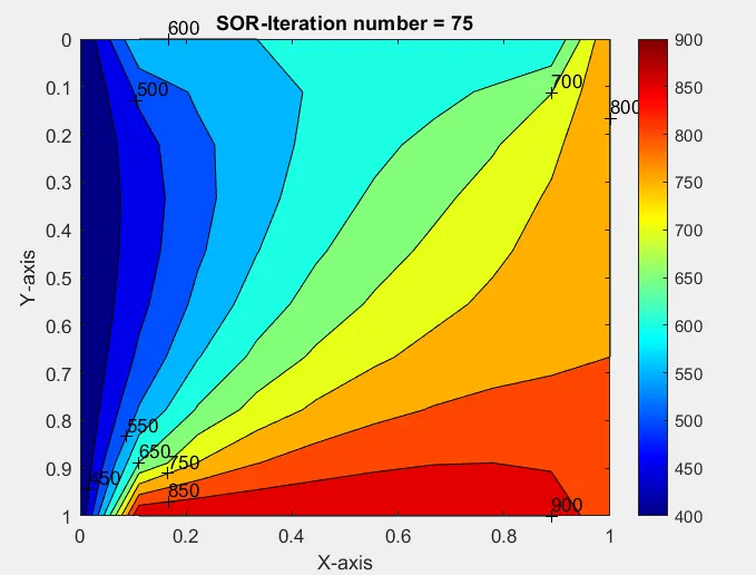
Errors:
error_Jacobi = 9.4868e-05
error_GS = 9.5865e-05
error_SOR = 8.2645e-05
No.of iterations:
Jacobi_iter = 207
gs_iter = 111
SOR_iter = 75
Elasped time:
- Elasped time for Jacobi method is 0.006982 seconds.
- Elasped time for GS method is 0.003197 seconds.
- Elasped time for SOR method is 0.003137 seconds.
From the observation, Jacobi > Gauss Seidel > SOR
i.e.; Jacobi method is taking more no.of iterations and the error value is also high.
Where as SOR method is taking less no.of iterations and also providing less error.
Transient state heat conduction:
General equation for the steady state 2D heat conduction is `(delT)/(delt)= alpha*[(del^2T)/(delx^2) +(del^2T)/(dely^2)]`
Where `T = Temperature (K)`
`x,y` are space coordinates
`t` = Time
In the Transient state 2D heat conduction there is a time term, So it can be solved either explicit method or implicit method.
The explicit and implicit methods are numerical analysis methods used to solve a time-dependent differential equations
Explicit method:
This method calculated the system status at a future time from the currently known system status.
In this method iterative methods are not used because all values are known. so that we can solve explicitly.
`T_P ^(n+1)= T_p^(n)+(k_1)*[T_L-(2*T_P)+T_R]+ (k_2)*[T_T-(2*T_P)+T_B]`
Applying the nodes (i,j) in the above equation
`implies``T_(i,j) ^(n+1)= T_(i,j)^(n)+(k_1)*[T_((i-1),j)-(2*T_(i,j)+T_((i+1),j))]^n+ (k_2)*[T_(i,(j-1))-(2*T_(i,j))+T_(i,(j+1))]^n`
MATLAB code for Transient state heat conduction ( Explicit Method):
%  UnSteady state analysis
%  Explicit method
clear all
close all
clc

% Defining inputs
nx=10; % No. of grid points along x axis
ny=10; % No. of grid points along y axis
% Define Mesh
x = linspace(0,1,nx);
y = linspace(0,1,ny);
% Mesh size
dx = x(2)-x(1);
dy = y(2)-y(1);
T=300*ones(nx, ny); % Initializing Temp.
% Applying boundry conditions
T(1,:)=600;     % Top Boundary
T(ny,:)=900; % Bottom Boundary
T(:,1)=400;   % Left Boundary
T(:,nx)=800; % Right Boundary

% Creating a copy
Told = T;
tol = 1e-4;
error = 10;
dt = 0.001;
alpha = 1.4;
Told = T;
% CFL number for x direction
k1 = alpha*(dt/dx^2);
% CFL number for y direction
k2 = alpha*(dt/dy^2);

tic
iter = 1;
for nt=1:1400
while(error>tol)
        % Space loop
        %for nt=1:1400
        for i= 2:nx-1
           for j= 2:ny-1
               % T(i,j) = (T^n)+k1*(T((i-1),j)-(2*T(i,j))+T((i+1),j))^n+k2*(T(i,(j-1))-(2*T(i,j))+T(i,(j+1)))^n;
               term1 = k1*(Told(i-1,j)-2*Told(i,j)+Told(i+1,j));
               term2 = k2*(Told(i,j-1)-2*Told(i,j)+Told(i,j+1));

               T(i,j) = T(i,j) + term1 + term2;
           end
        end
        error= max(max(abs(Told-T)));
        Told=T; % Updating Told value
        iter = iter+1;
        end

end
 % Plotting
 figure(1)
 contourf(x,y,T)
 clabel(contourf(x,y,T));
 colorbar
 colormap(jet)
 xlabel('X-axis')
 ylabel('Y-axis')
 title_text = sprintf('iteration number = %d',iter);
 title(title_text)
 set(gca,'YDIR','reverse')
toc
Simulation Results:
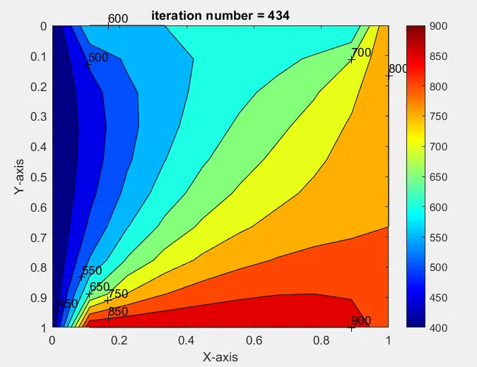
- No. of iterations = 434.
- Error = 9.883610562155809e-05
- CFL number = 0.2268.
- Since CFL < 0.5, the solution is stable.
- Elapsed time is 0.699258 seconds.
Implicit method:
This method calculates the system status at a future time from the system status at present and future times.
In this method iteretive methods are used because all values are unknowns.
`T_P ^(n+1)= (1/(1+2k_1+2k_2))*[T_p^(n)+(k_1)*(T_L+T_R)^(n+1)+ (k_2)*(T_T-(2*T_P)+T_B)^(n+1)]`
Applying the nodes (i,j) in the above equation
`implies``T_(i,j) ^(n+1)= (1/(1+2k_1+2k_2))*[T_(i,j)^(n)+(k_1)*(T_((i-1),j)+T_((i+1),j)))^(n+1)+ (k_2)*(T_(i,(j-1))-(2*T_(i,(j+1))+T_B)^(n+1)]`
MATLAB code for Transient state heat conduction ( Implicit Method):
%  UnSteady state analysis
%  Implicit method
clear all
close all
clc

% Defining inputs
nx=10; % No. of grid points along x axis
ny=10; % No. of grid points along y axis
% Define Mesh
x = linspace(0,1,nx);
y = linspace(0,1,ny);
% Mesh size
dx = x(2)-x(1);
dy = y(2)-y(1);
T=300*ones(nx, ny); % Initializing Temp.
% Applying boundry conditions
T(1,:)=600;     % Top Boundary
T(ny,:)=900;      % Bottom Boundary
T(:,1)=400;      % Left Boundary
T(:,nx)=800;     % Right Boundary

% Creating a copy
Told = T;
Tinitial = T;
T_prev = Told;

tol = 1e-4;
dt = 0.001;
alpha = 1.4;


% CFL number for x
k1 = alpha*(dt/dx^2);
% CFL number for y
k2 = alpha*(dt/dy^2);

 tic
% % Jacobi method
Implicit_Jacobi_iter = 0;

  % Time loop
 for nt=1:1400
     % Convergence loop
     error_Jacobi = 10;
     while(error_Jacobi>tol)
          % Space loop
        for i= 2:nx-1
           for j= 2:ny-1
               term1 = 1/(1+2*k1+2*k2);
               term2 = k1*term1;
               term3 = k2*term1;
               H = Told(i-1,j)+Told(i+1,j);
               V = Told(i,j-1)+Told(i,j+1);

               T(i,j) =(term1*T_prev(i,j))+(H*term2)+(V*term3);
           end
        end
        error_Jacobi= max(max(abs(Told-T)));
        Told=T; % Updating Told value
        Implicit_Jacobi_iter = Implicit_Jacobi_iter+1;
        end
        T_prev = T;
 end
toc

%  % Plotting
 figure(1)
 contourf(x,y,T)
 clabel(contourf(x,y,T));
 colorbar
 colormap(jet)
 xlabel('X-axis')
 ylabel('Y-axis')
 title_text = sprintf('Implicit-Jacobi-Iteration number = %d',Implicit_Jacobi_iter);
 title(title_text)
 set(gca,'YDIR','reverse')


% % Gauss seidel method

T=300*ones(nx, ny); % Initializing Temp.
% Applying boundry conditions
T(1,:)=600;     % Top Boundary
T(ny,:)=900;      % Bottom Boundary
T(:,1)=400;      % Left Boundary
T(:,nx)=800;     % Right Boundary
% Creating a copy
Told = T;
Tinitial = T;
T_prev = Told;
tic
Implicit_GS_iter = 0;
     % Time loop
 for nt=1:1400
     error_GS = 10;
     %   Convergence loop
     while(error_GS>tol)
         % Space loop
        for i= 2:nx-1
           for j= 2:ny-1
               term1 = (1+2*k1+2*k2)^-1;
               term2 = k1*term1;
               term3 = k2*term1;
               H = T(i-1,j)+Told(i+1,j);
               V = T(i,j-1)+Told(i,j+1);

               T(i,j) =(term1*T_prev(i,j))+(H*term2)+(V*term3);
           end
        end
        error_GS= max(max(abs(Told-T)));
        Told=T; % Updating Told value
        Implicit_GS_iter = Implicit_GS_iter+1;
        end
        T_prev = T;
 end
toc

%  % Plotting
 figure(2)
 contourf(x,y,T)
 clabel(contourf(x,y,T));
 colorbar
 colormap(jet)
 xlabel('X-axis')
 ylabel('Y-axis')
 title_text = sprintf('Implicit-GS-Iteration number = %d',Implicit_GS_iter);
 title(title_text)
 set(gca,'YDIR','reverse')


 % SOR method

T=300*ones(nx, ny); % Initializing Temp.
% Applying boundry conditions
T(1,:)=600;     % Top Boundary
T(ny,:)=900;      % Bottom Boundary
T(:,1)=400;      % Left Boundary
T(:,nx)=800;     % Right Boundary
% Creating a copy
Told = T;
Tinitial = T;
T_prev = Told;
w = 1.1;
tic
Implicit_SOR_iter = 0;
% Time loop
 for nt=1:1400
     % Convergence loop
    error_SOR = 10;
     while(error_SOR>tol)
          % Space loop
        for i= 2:nx-1
           for j= 2:ny-1
               term1 = (1+2*k1+2*k2)^-1;
               term2 = k1*term1;
               term3 = k2*term1;
               H = T(i-1,j)+Told(i+1,j);
               V = T(i,j-1)+Told(i,j+1);

               T(i,j) =(1-w)*Told(i,j)+w*(term1*T_prev(i,j)+(H*term2)+(V*term3));
           end
        end
        error_SOR= max(max(abs(Told-T)));
        Told=T; % Updating Told value
        Implicit_SOR_iter = Implicit_SOR_iter+1;
     end
        T_prev = T;
 end
toc

 % Plotting
 figure(3)
 contourf(x,y,T)
 clabel(contourf(x,y,T));
 colorbar
 colormap(jet)
 xlabel('X-axis')
 ylabel('Y-axis')
 title_text = sprintf('Implicit-SOR-Iteration number = %d',Implicit_SOR_iter);
 title(title_text)
 set(gca,'YDIR','reverse')
Simulation Results:
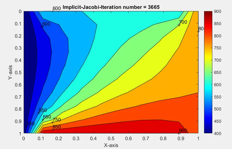
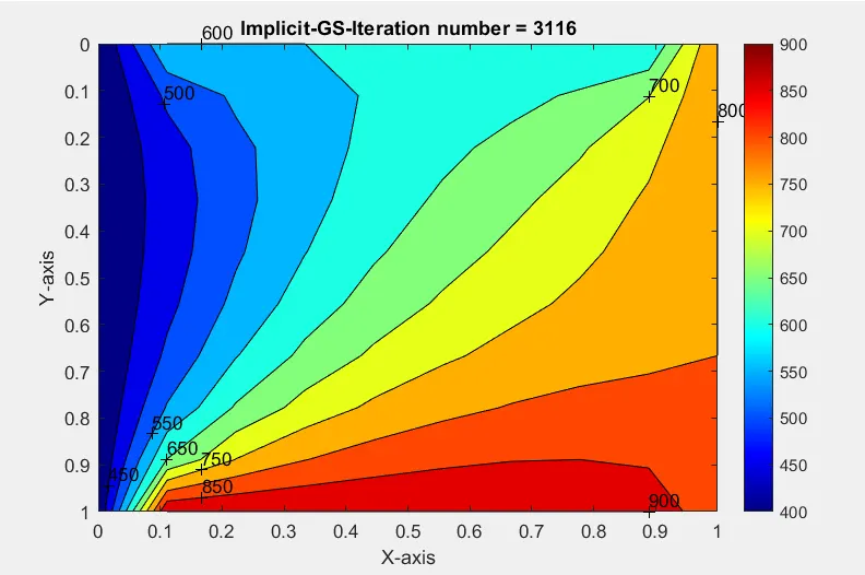
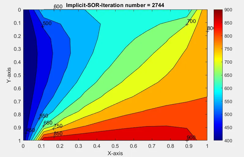
- Contours of Jacobi, Gauss seidel and SOR iterations:
Error:
- error_Jacobi = 1.250555214937776e-12
- error_GS = 0
- error_SOR = 1.136868377216160e-13
Iterations:
- No. of iterations for Jacobi method is 3665
- No. of iterations for GS method is 3116
- No. of iterations for SOR method is 2744
Elasped time:
- Elasped time for Jacobi method is 0.018115 seconds.
- Elasped time for GS method is 0.017823 seconds.
- Elasped time for SOR method is 0.017378 seconds.
From the observation, Jacobi > Gauss Seidel > SOR
i.e.; Jacobi method is taking more no.of iterations and the error value is also high.
Where as SOR method is taking less no.of iterations and also providing less error.