Week 5 - Mid term project - Solving the steady and unsteady 2D heat conduction problem
AIM : To solve the steady and unsteady 2-D Heat conduction equation using implicit and explicit methods in MATLAB
INTRODUCTION :
In oder to achieve the objective of this program we have to understand some concepts in detail . lets have a look on them :
1. Thermal conduction : Thermal conduction can be defined as the transfer of internal energy by microscopic collisions and movement of electrons.
2. steady state heat conduction : steady state heat conduction is a form of conduction when the temperature difference driving the conduction are constant , ie the temperature is not changing with respect to time . Thus the spatial distribution in the conduction object does not changes and it is equated to 0 . Thus in steady state the ammount of heat entering the body is equal to the ammount of heat leaving out of the body. The equation can be stated as :
`(partial^2T)/(partialx^2) +(partial^2T)/(partialy^2) = 0`..................(1)`
3. Transient Equation : Transient equation in simple words can be said as the change of the steady state equation with respect to time . This can be also said as unsteady or transient equation, the quation can be stated as :
`(partial T)/(partialt)= alpha((partial^2T)/(partialx^2) + (partial^2T)/(partialy^2))`........(2)
`alpha =`it is known as diffusive co-effecient , which is the ratio of thermal conductivity to the product of specific heat capacity at constant pressure and density , the formula is as follows :
`alpha = k/(rho*c_p)`..........(3)`
STEADY STATE HEAT CONDUCTION EQUATION :
In this project we are going to solve the steady state equation implicity with the help of iterative solvers :
1). jacobi method
2). Gauss seidel method
3). Sucessive over relaxation method
Math behind :
`(partial^2T)/(partialx^2) +(partial^2T)/(partialy^2) = 0`...........(4)
this is a partial derrivative equation , lets solve it implicitly using the iterative solvers , The equation 4 is a symetric quation which means in oder to solve the steady state equation we are taking the information from the points symetrically about the initial point as shown in the figure 1.
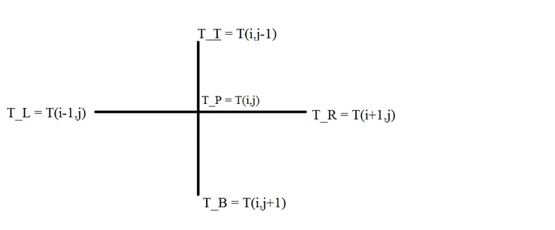
Figure 1: grid spacing
Equation 4 can be solved using a central difference scheme by taking the information equally from the points ahead and back of the initial point in both x and y direction . The grid spacing between the points in x and y directions are given as x^2 and y^2 respectively . The central difference scheme for the equation 4 can be written as :
`(T_L-2T_P+T_R)/(trianglex^2) + (T_T-2T_P+T_B)/(triangley^2) =0`...................(6)
`(T_L + T_R)/(trianglex^2) +(T_T+T_B)/(triangley^2)=T_P ( 2/(trianglex^2)+2/(triangley^2))`................(7)
we are defining a variable k to simplify the equation (6)
`2/(trianglex^2)+2/(triangley^2) = k`..................(8)
Now when we substitute equation (8) to equation (7) and simplify we get :
`T_P = 1/K*((T_L+T_R)/(trianglex^2) + (T_T+T_B)/(triangley^2))`...................(9)
eq (9) is used in the iterative solvers to find out the steady state error but we can simplify it more we know that the grid spacing is same and equal so we can say that
`trianglex^2 = triangley^2`.................(10)
Now substituting equation (10) in equation (9) and simplifying we get :
`T_P = 1/4 *(T_L+T_R+T_T+T_B)`......(11)
Thus we are using equation 11 in the iterative solvers to solve the steady state equation .
lets look at the iterative solvers in detail :
ITERATIVE SOLVERS :
jacobi method :
Jacobi method is a iterative solver based on numerical methods where we estimate an initial value and keep on iterating until we get the value of `(n+1)^(th)` iteration is equal to `n^(th)` iteration , lets look at it in more detail to understand it in a betterway.
`5x +3y+ 4z = 15`
`12x+13y+8z = 40`
`15 x +20y+10z = 110`
so first we have check that the sum of diagonal matrix is greater then the sum of other two terms then we procced to find out the values of x , y and z , which is as follows :
`x = 1/5*(15-3y+4z)`...........(12)
`y = 1/13*(40-12x-8z)`.........(13)`
`z= 1/10*(110-15x-20y)`..........(14)
now for 1 st iteration we are substituting 0,0,0 to find out the values of x, y, z from eq(12),eq(13) and eq(14) respectively , now in second iteration we are substituting the values which we get in 1 st iteration so this is the jacobi method . The formula used to calculate the Temperature at point T(i,j) in this program can be given as :
`T(i,j) = 0.25 *(T_(old)(i-1,j)+ T_(old)(i+1,j)+ T_(old)(i,j-1)+ T_(old)(i,j+1))`................(15)
Gauss seidel equation :
The proccedure and concept in the gauss seidel iteration is same as jacobi method but there is a small change , In gauss seiedel method we have to add the new values in the imeediate iteration for example :
we are performimg the first iteration by giving the estimated values for x , y and z to find out x , then new value of x is used to find out the values of y and z from equation 13 and 14 in the first iteration itself , when we are finding out the value of z in equation 14 for 1 st iteration we are using the new values of x and y . The same proccedure is repeated for 2nd iteration and so on , The equation converges when nth iteration (last iteration ) is aproximately similar to (n-1)th iteration.
The formula used to calculate the Temperature at point T(i,j) in this program can be given as :
`T(i,j) = 0.25 *(T(i-1,j)+ T_(old)(i+1,j)+ T(i,j-1)+ T_(old)(i,j+1))`.................................(16)
Sucessive over relaxation method :
This the method where we use the change in slope of the values with respect to the iteration along with a relaxation factor , so the formula for the sucessive relaxation used in this program can be given as :
`T(i,j) = ((1- omega)*T_(old)(i,j)+ (omega*0.25*(T(i-1,j)+ T_(old)(i+1,j)+ T(i,j-1)+ T_(old)(i,j+1))));`.............(17)
here we use the value of `omega` = 1.2
Input values :
L =1
nx = 30 ( do define the number of grid points )
ny = nx
x = linspace(0,l,nx)
same way define the y values
Top Boundary = 600 K
Bottom Boundary = 900 K
Left Boundary = 400 K
Right Boundary = 800 K
Proccedure :
1. Use the close all , clear all and clc command to clear the work space .
2. Now lets define the input values , grid points and all the necessary requirements .
3. In this program we are solving the steady state - heat conduction equation using the iterative solvers so we have to define 3 for loops for 3 iterative solvers respectively.
4. Now we have to define a if statement for each for loop , ie for example '' for iterative solver==1 , if iterative solver ==1 , then the formula is '' jacobi method (defining the formula as derived earlier)'''.
5. so create a if loop for the respective solvers and assign the formulas derrived in eqation (15),(16) and (17) respectively , inside the for loop and if loop of the respective solvers .
6. compute the formula in sucha a way that the equation runs for all the inner grid points of the matrix [nx.ny]
7. The iterations should run until the equation is converged for that we are assigning a tollerance value and using a while loop , ie the solver will run till a point when the error value reaches below the iteration value , at this point it means the equation is converged .
8. now we are updating the error value after the while loop, using the max command .
9. Now we are closing the loops and plotting the contour plots for each solvers , The steps are repeated for each solvers .
code :
% program to evaluate the steady state heat transfer equation
close all
clear all
clc
% Equation : d^2 T/ dx^2 + d^2 T/ dy^2 = 0
% Inputs :
l = 1 ; % length of the domain
% No of grid points along x and y direction
nx = 30 ;
ny = nx ;
x = linspace(0,1,nx);
y = linspace(0,1,ny);
dx = x(2)-x(1);
dy = y(2)-y(1);
error = 9e9 ;
tol = 1e-4 ; % tollerance value
% Defining the boundry conditions
T_L = 400 ;
T_R = 800 ;
T_T = 600 ;
T_B = 900 ;
T = ones(nx,ny);
% calculation of the relaxation factor
omega = 1.2;
% Temperature at boundry
T(2: nx-1 , 1) = T_L ;
T(2: nx-1 , ny) = T_R ;
T(1,2 : ny-1) = T_T ;
T(nx,2:ny-1) = T_B   ;
% defining the temperatures at the corner points
T(1,1) = ((T_L + T_T)/2);
T(nx,1) = ((T_L + T_B)/2) ;
T(1,ny) = ((T_T + T_R)/2);
T(nx,ny)= ((T_R +T_B)/2);
% creating a copy of T
[X,Y] = meshgrid(x,y);
T_old = T ;
% Jaccobi method
for iter_solver = 1
    tic ;
    if iter_solver == 1
        jacobi_iteration = 1 ;
        while (error > tol)
            for i = 2: nx-1
                for j = 2: ny-1
                    T(i,j) = 0.25 *(T_old(i-1,j)+ T_old(i+1,j)+ T_old(i,j-1)+ T_old(i,j+1));
                end
            end
            error = max(max(abs(T_old -T)));
            T_old = T;
            jacobi_iteration = jacobi_iteration + 1;
        end
    end
            F = toc ;
            % plotting
            figure(1);
            [p,q] = contourf(X,Y,T);
            clabel(p,q);
            colormap(jet) ;
            colorbar ;
            set(gca,'YDIR','reverse')
            title_text = sprintf('Jacobi Method , Iteration number = %d, computation time F=%fs',jacobi_iteration ,F);
            title(title_text);
            xlabel('xaxis');
            ylabel('yaxis') ;
            fprintf( 'No of iterations in jacobi method =%dn',jacobi_iteration);
            pause (0.03 )
end
% gauss seiedel method
for iter_solver = 2
    % updated values
    l = 1 ; % length of the domain
% No of grid points along x and y direction
    nx = 30 ;
    ny = nx ;
    x = linspace(0,1,nx);
    y = linspace(0,1,ny);
    dx = x(2)-x(1);
    dy = y(2)-y(1);
   error = 9e9 ;
   tol = 1e-4 ; % tollerance value
% Defining the boundry conditions
      T_L = 400 ;
      T_R = 800 ;
      T_T = 600 ;
      T_B = 900 ;
      T = 300*ones(nx,ny);
% Temperature at boundry
T(2: nx-1 , 1) = T_L ;
T(2: nx-1 , ny) = T_R ;
T(1,2 : ny-1) = T_T ;
T(nx,2:ny-1) = T_B   ;
% defining the temperatures at the corner points
T(1,1) = ((T_L + T_T)/2);
T(nx,1) = ((T_L + T_B)/2) ;
T(1,ny) = ((T_T + T_R)/2);
T(nx,ny)= ((T_R +T_B)/2);
  % creating a copy of T
     [X,Y] = meshgrid(x,y);
     T_old = T ;

    tic ;
    if iter_solver == 2
        gs_iteration = 1 ;
        while (error > tol)
            for i = 2: nx-1
                for j = 2: ny-1
                    T(i,j) = 0.25 *(T(i-1,j)+ T_old(i+1,j)+ T(i,j-1)+ T_old(i,j+1));
                end
            end
            error = max(max(abs(T_old -T)));
            T_old = T;
            gs_iteration = gs_iteration + 1;
        end
    end
          F = toc ;
            % plotting
            figure(2);
            [p,q] = contourf(X,Y,T);
            clabel(p,q);
            colormap(jet) ;
            colorbar ;
            set(gca,'YDIR','reverse')
            title_text = sprintf('Gauss seidel , Iteration number = %d, computation time F=%fs',gs_iteration ,F);
            title(title_text);
            xlabel('xaxis');
            ylabel('yaxis') ;
            fprintf( 'No of iterations in gauss_seidel method =%dn',gs_iteration);
            pause (0.03 )
end
 % sor method
 for iter_solver = 3
    % updated values
    l = 1 ; % length of the domain
% No of grid points along x and y direction
    nx = 30 ;
    ny = nx ;
    x = linspace(0,1,nx);
    y = linspace(0,1,ny);
    dx = x(2)-x(1);
    dy = y(2)-y(1);
   error = 9e9 ;
   tol = 1e-4 ; % tollerance value
% Defining the boundry conditions
      T_L = 400 ;
      T_R = 800 ;
      T_T = 600 ;
      T_B = 900 ;
      T =  250*ones(nx,ny);
      % calculation of the relaxation factor
      omega = 1.2 ;
% Temperature at boundry
T(2: nx-1 , 1) = T_L ;
T(2: nx-1 , ny) = T_R ;
T(1,2 : ny-1) = T_T ;
T(nx,2:ny-1) = T_B   ;
% defining the temperatures at the corner points
T(1,1) = ((T_L + T_T)/2);
T(nx,1) = ((T_L + T_B)/2) ;
T(1,ny) = ((T_T + T_R)/2);
T(nx,ny)= ((T_R +T_B)/2);
  % creating a copy of T
     [X,Y] = meshgrid(x,y);
     T_old = T ;

    tic ;
    if iter_solver == 3
        sor_iteration = 1 ;
        while (error > tol)
            for i = 2: nx-1
                for j = 2: ny-1
                    T(i,j) = ((1- omega)*T_old(i,j)+ (omega*0.25*(T(i-1,j)+ T_old(i+1,j)+ T(i,j-1)+ T_old(i,j+1))));
                end
            end
            error = max(max(abs(T_old -T)));
            T_old = T;
            sor_iteration = sor_iteration + 1;
        end
    end
          F = toc ;
            % plotting
            figure(3);
            [p,q] = contourf(X,Y,T);
            clabel(p,q);
            colormap(jet) ;
            colorbar ;
            set(gca,'YDIR','reverse')
            title_text = sprintf(' sor , Iteration number = %d, computation time F=%fs',sor_iteration ,F);
            title(title_text);
            xlabel('xaxis');
            ylabel('yaxis') ;
            fprintf( 'No of iterations in sucessive over relaxation method =%d n',sor_iteration);
            pause (0.03 )
end
Figure 2 : steady state equation solver
Results plot :
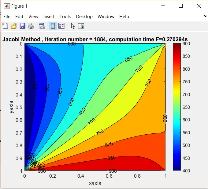
Figure 1 : Jacobi method
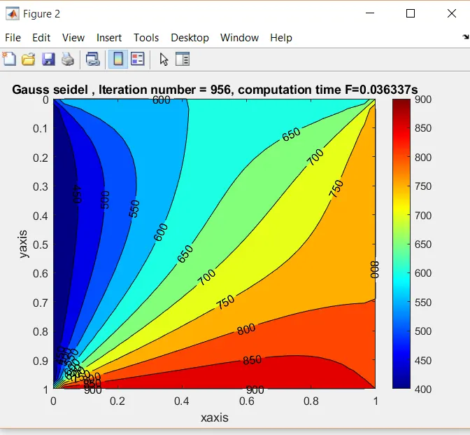
Figure 3 : Gauss- seiedel method
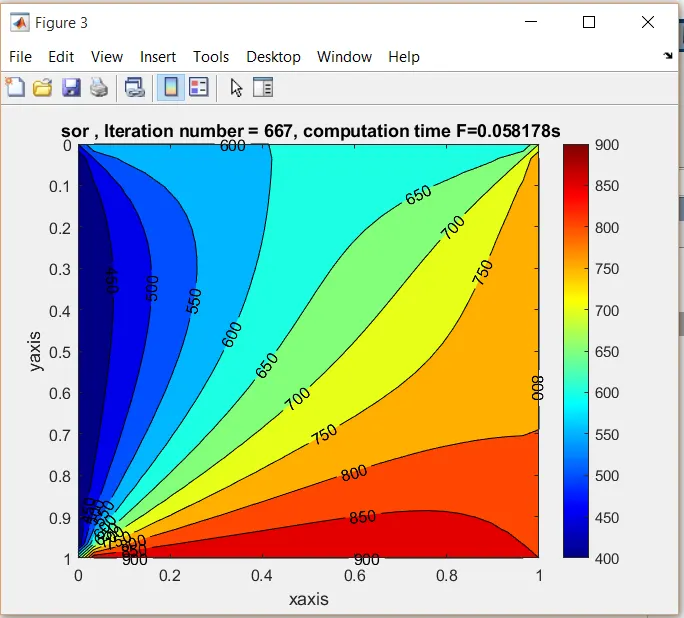
Figure 4 : Sucessive over relaxation method
No of iterations in jacobi method =1884
No of iterations in gauss_seidel method =956
No of iterations in sucessive over relaxation method =667
>>
Figure 5 : No of iterations
From figure 3,4 and 5 we can say that the computing time is higher for the jacobi method and the no of iterations is also higher for the jacobi method and the iterationand computing time is lower for the sucessive over relaxation method , the oder of iterations is as follows :
Jacobi method > Gauss seiedel method > Sucessive over relaxation method
TRANSIENT HEAT CONDUCTION EQUATION :
From the previous section we know that the transient heat conduction equation is as follows :
`(dT)/dt - alpha((d^2 T)/ dx^2 + (d^2 T)/ dy^2) = 0`..................(18)
This equation can be solved in two different ways the explicit method and the implicit method which are as follows ;
Explicit method :
`(dT)/dt = alpha((d^2 T)/ dx^2 + (d^2 T)/ dy^2)`....................(19)
Now lets use taylors table expansion to solve this equation explicitly , and use the Temperature equations as in figure 1 :
`(T_P^(n+1)-T_p^n)/(partialt) = alpha[(T_L-2T_P+T_r)/(partialx^2) + (T_T-2T_P+T_B)/(partialy^2)]`......................(20) `
Now this equation is solved using a time marching proccedure and if its a explicit equation , we are powering the RHS to the power of n , Which means we are calculating the Temperature at Time step 2 using the Temperature at Time step 1 , this known as explicit method and it is as follows :
`(T_P^(n+1)-T_p^n)/(partialt) = alpha[(T_L^n-2T_P^n+T_R^n)/(partialx^2) + (T_T^n-2T_P^n+T_B^n)/(partialy^2)]`.....................(21)
we simplify this equation by defining two constants :
`k_1 = (alpha*partialt)/(partialx^2)`....................(22`
`k_2 = (alpha*partialt)/(partialy^2)`....................(23)
So now the equation 21 becomes as follows :
`T_p^(n+1) = T_p^n+k_1(T_L^n -2*T_p^n +T_R^n)+k_2(`T_T^n -2*T_p^n +T_B^n`)`.....(22)
lets simplify it more by dividing the terms :
Term_1 = `T_L^n -2*T_p^n +T_R^n`...................(23)
Term_2 = `T_T^n -2*T_p^n +T_B^n`...................(24)
Now substituting the equations 23 and 24 in eq 22 we get the equation as follows :
`T_p^(n+1) = T_p^n+k_1(term_1)+k_2(term_2)`...........(25)
equation 25 is used to solve the Transient analysis equation explicitly
Implicit method :
In simple words implicit analysis is the method where we solve the equation using the time marching method by using the information in the current time step and previous time step combinedly lets look at it in detail as shown below :
`T_p^(n+1) = T_p^n+k_1(T_L^(n+1) -2*T_p^(n +1)+T_R^(n+1))+k_2(T_T^(n+1) -2*T_p^(n +1)+T_B^(n+1))`............(26)
Now lets re-arrange the equation (26) in a simpler way by keeping the T(i,j) at the (n+1) time step on one side as follows :
`T_P^(n+1)+2*k_1*T_P^(n+1) +2*k_2*T_P^(n+1) = T_P^n+ k_1(T_L^(n+1)+T_R^(n+1))+k_2(T_T^(n+1)+T_B^(n+1))`............(27)
`T_P^(n+1) = 1/(1+2*k_1+2k_2)*(T_P^n+ k_1(T_L^(n+1)+T_R^(n+1))+k_2(T_T^(n+1)+T_B^(n+1)))`...................(28)
Now lets simplify the equation more :
term_1 = `1/(1+2*k_1+2k_2)`................(29)
term_2 = `term_1*k_1`........................(30)
term_3 = `term_1*k_2`...........................(31)
H = `T_L^(n+1)+T_R^(n+1)`..............(32)
V= `T_T^(n+1)+T_B^(n+1)`...............(33)
Now substitute the equation (29),(30),(31),(32) and (33) in equation 28 and we get :
`T_P^(n+1) = T_P^(n)*term_1+ H*term_2 +V*term_3`................(34)`
Now this equation is used to solve the transient heat conduction equation using the iterative solvers , here `T_P^n` it is temperature at the present point at previous time step denoted by `T_(prev)`. Now this equation (34) is incorporated into the iterative solvers jacobi, gauss seiedel and sucessive over relaxation method , In the previous sections we have looked more about derriving the iterative solvers , so now lets look at the formulas for the iterative solvers which is as follows :
Jacobi method :
For each iterative solvers there will be slight changes in the term H and V , which are as follows :
`H = T_(old)(i-1,j)+ T_(old)(i+1,j)`..................(35)
`V = T_(old)(i,j-1) + T_(old)(i,j+1)`................(36)
`(i,j)=(T_(prev)(i,j)*term_1)+( H * term_2)+( V*term_3)..................(36`
The terms , '' term_1 , term_2 and term_3 are same for all the iterative solvers .
Gauss-siedel method :
For each iterative solvers there will be slight changes in the term H and V , which are as follows :
`H = T(i-1,j)+ T_(old)(i+1,j)`.........................(37)
`V = T(i,j-1) + T_(old)(i,j+1)`.........................(38)
`T(i,j)=(T_(prev)(i,j)*term_1)+( H * term_2)+( V*term_3)`.................(39)
The terms , '' term_1 , term_2 and term_3 are same for all the iterative solvers .
Sucessive over relaxation method :
In this method we are using the gauss-siedel method to find the slope of errors for sucessive over relaxation method :
`H = T(i-1,j)+ T_(old)(i+1,j)`.............(40)
`V = T(i,j-1) + T_(old)(i,j+1)`.............(41)
`T(i,j)= ((1-omega)*T_(old)(i,j)+ (omega*((T_(prev)(i,j)*term_1)+(H*term_2)+(V*term_3))))`..................(42)
The terms , '' term_1 , term_2 and term_3 are same for all the iterative solvers .
Proccedure (Explicit method ):
1. Use the close all , clear all and clc command to clear the work space .
2. Now lets define the input values , grid points and all the necessary requirements .
3. In this program we are solving the Transient heat conduction equation using the explicit method.
4. since we are solving this method using a time marching proccedure , first we have to define a time loop saying " for time_step = 1: no of time step ''. Then we have to make a convergence loop for the steady state equation .
5. Then comes our while loop to define the no of iteration till which the solver should run .
6. Inside the while loop we are defining the convergence loop '' for i = 2: nx-1 and for j = 2:ny-1'' . Then we define our formula for the explicit method and end the for loop .
7. Error values are updated after the end of while loop then the if loop is brought to an end .
8. The `T_(old)` is updated before the end of the time loop .
9. Now use the contourf and printf command to plot the contour plot and no of iterations .
10. now end the loops
11. End the program
Proccedure (Implicit Method ) :
1. Use the close all , clear all and clc command to clear the work space .
2. Now lets define the input values , grid points and all the necessary requirements .
3. In this program we are solving the Transient heat conduction equation using the Implicit method.
4. since we are solving this method using a time marching proccedure , first we have to define a time loop saying " for time_step = 1: no of time step ''. Then we have to make a convergence loop for the steady state equation .
5. Then comes our if loop and while loop to define to solver and the no of iteration till which the solver should run .
6. Inside the while loop we are defining the convergence loop '' for i = 2: nx-1 and for j = 2:ny-1'' . Then we define our formula for the explicit method and end the for loop .
7. Now we have repeat the steps (5) and (6) for the other two iterative solvers gauss seiedel and sucessive over relaxation method respectively.
8. Error values are updated after the end of while loop then the if loop is brought to an end .
9. The `T_(prev)` is updated before the end of the time loop .
10. Now end the time loop and use the contourf and printf command to plot the contour plot and no of iterations .
11. End the program
code :
% To solve the transient heat conduction equation using Explicit method
close all
clear all
clc
% Equation : dT/dt - alpha(d^2 T/ dx^2 + d^2 T/ dy^2) = 0
% Inputs :
l = 1 ; % length of the domain
% No of grid points along x and y direction
nx = 12;
ny = nx ;
x = linspace(0,1,nx);
y = linspace(0,1,ny);
dx = l/(nx-1);
dy = l/(ny-1);
alpha = 1.4 ; % Thermal diffusivity value
nt = 1400 ; % no of time steps
dt = 0.001 ;% time step
error = 9e9 ;
tol = 1e-4 ; % tollerance value
k1 = ((alpha*dt)/(dx^2)) ;
k2 = ((alpha*dt)/(dy^2)) ;
% Defining the boundry conditions
T_L = 400 ;
T_R = 800 ;
T_T = 600 ;
T_B = 900 ;
T = ones(nx,ny);
% calculation of the relaxation factor
omega = 1.2 ;
% Temperature at boundry
T(2: nx-1 , 1) = T_L ;
T(2: nx-1 , ny) = T_R ;
T(1,2 : ny-1) = T_T ;
T(nx,2:ny-1) = T_B   ;
% defining the temperatures at the corner points
T(1,1) = ((T_L + T_T)/2);
T(nx,1) = ((T_L + T_B)/2) ;
T(1,ny) = ((T_T + T_R)/2);
T(nx,ny)= ((T_R +T_B)/2);
% creating a copy
[X , Y] = meshgrid(x,y);
T_old = T;
CFL = k1 + k2
unsteady_explicit_iter = 1;
tic
for time_loop = 1: nt
    while(error>tol)
        for i = 2: nx-1
            for j = 2: nx-1
                term_1 = T_old(i-1,j)- (2*T_old(i,j))+ T_old(i+1,j);
                term_2 = T_old(i,j-1)- (2*T_old(i,j))+ T_old(i,j+1);
                T(i,j) = T_old(i,j)+ (k1*term_1)+ (k2*term_2);
            end
        end
        error = max(max(abs(T_old-T)));
        T_old = T ;
        unsteady_explicit_iter = unsteady_explicit_iter +1 ;
         figure(1)
        [P,Q] = contourf(X,Y,T);
        set(gca,'YDIR','reverse')
        colorbar
        colormap(jet)
        clabel(P,Q);
        text = sprintf( 'Unsteady Explicit Iterations = %d',unsteady_explicit_iter);
        xlabel('X')
        ylabel('y')
        title(text)
        pause(0.03)

    end
end
 % plot

        fprintf( 'No of iterations in Explicit method =%d n',unsteady_explicit_iter);

        time_taken = toc
Figure 6: Program code for Explicit method
Results and plots :
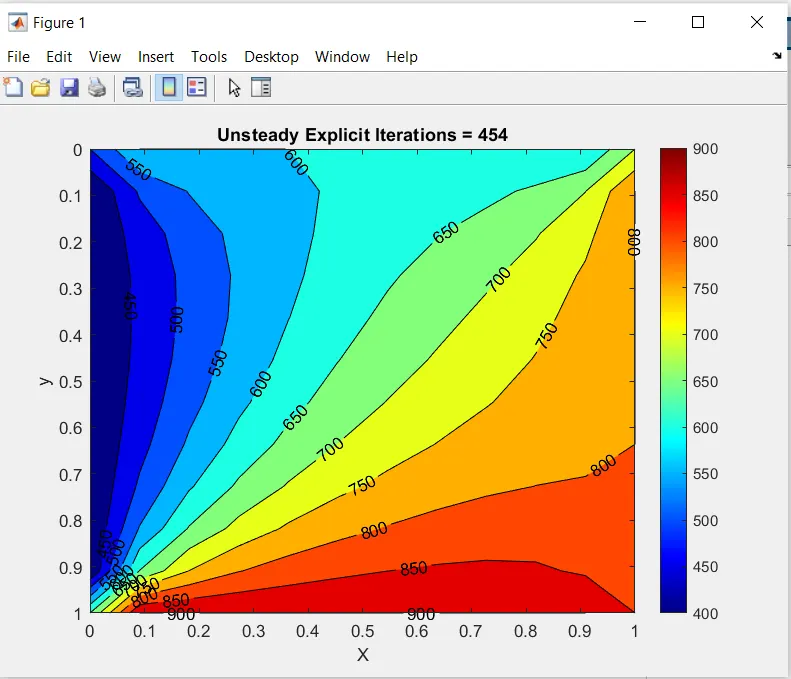
Figure 7 : Unsteady heat conduction equation Explicit method
CFL =

    0.3388

No of iterations in Explicit method =454

time_taken =

   95.4623
Figure 8 : Result output for explicit method
Code (Implicit method ) :
% program to evaluate the un-steady state heat transfer equation or transient equation

close all
clear all
clc
% Equation : dT/dt - alpha(d^2 T/ dx^2 + d^2 T/ dy^2) = 0
% Inputs :
l = 1 ; % length of the domain
% No of grid points along x and y direction
nx = 15 ;
ny = nx ;
x = linspace(0,1,nx);
y = linspace(0,1,ny);
dx = l/(nx-1);
dy = l/(ny-1);
alpha = 1.4 ; % Thermal diffusivity value
nt = 1500 ; % no of time steps
dt = 0.001 ;% time step
error = 9e9 ;
tol = 1e-4 ; % tollerance value
k1 = ((alpha*dt)/(dx^2)) ;
k2 = ((alpha*dt)/(dy^2)) ;

% Defining the boundry conditions
T_L = 400 ;
T_R = 800 ;
T_T = 600 ;
T_B = 900 ;
T = ones(nx,ny);
% calculation of the relaxation factor
omega = 1.2 ;
% Temperature at boundry
T(2: nx-1 , 1) = T_L ;
T(2: nx-1 , ny) = T_R ;
T(1,2 : ny-1) = T_T ;
T(nx,2:ny-1) = T_B   ;
% defining the temperatures at the corner points
T(1,1) = ((T_L + T_T)/2);
T(nx,1) = ((T_L + T_B)/2) ;
T(1,ny) = ((T_T + T_R)/2);
T(nx,ny)= ((T_R +T_B)/2);
 % creating a copy of T
     T_old = T ;
     T_prev_dt = T ; % copy for previous time step
     iter =1 ;
      iterative_solver = input('1) jacobi method 2) Gauss seidel 3)Sucessive over relaxation n Enter an option for the type of solver u want to use : n ');
      tic
      for time_step = 1: nt
          if iterative_solver == 1
              term_1 = ( 1+ 2*k1 + 2*k2)^-1 ;
              term_2 = term_1*k1 ;
              term_3 = term_1*k2 ;
              error =9e9;
              while(error>tol)
                  for i = 2:nx-1
                      for j = 2:ny-1
                          H = (T_old(i-1,j)+ T_old(i+1,j));
                          V = (T_old(i,j-1) + T_old(i,j+1));
                          T(i,j)=(T_prev_dt(i,j)*term_1)+( H * term_2)+( V*term_3);
                      end
                  end

                  error = max(max(abs(T_old - T)));
                  T_old = T;
                  iter = iter+1 ;
              end

           end
           if iterative_solver ==2
              term_1 = ( 1+ 2*k1 + 2*k2)^-1 ;
              term_2 = term_1*k1 ;
              term_3 = term_1*k2 ;
              error =9e9;
              while(error>tol)
                  for i = 2:nx-1
                      for j = 2:ny-1
                          H = (T(i-1,j)+ T_old(i+1,j));
                          V = (T(i,j-1) + T_old(i,j+1));
                          T(i,j)=(T_prev_dt(i,j)*term_1)+( H * term_2)+( V*term_3);
                      end
                  end
                  error = max(max(abs(T_old - T)));
                  T_old = T;
                  iter = iter+1 ;
              end

           end
          if iterative_solver ==3
              term_1 = ( 1+ 2*k1 + 2*k2)^-1 ;
              term_2 = term_1*k1 ;
              term_3 = term_1*k2 ;
              error =9e9;
              while(error>tol)
                  for i = 2:nx-1
                      for j = 2:ny-1
                          H = (T(i-1,j)+ T_old(i+1,j));
                          V = (T(i,j-1) + T_old(i,j+1));
                          T(i,j)= ((1-omega)*T_old(i,j)+ (omega*((T_prev_dt(i,j)*term_1)+(H*term_2)+(V*term_3))));
                      end
                  end
                  error = max(max(abs(T_old - T)));
                  T_old = T;
                  iter = iter+1 ;
              end

          end
          T_prev_dt = T ;

      end
      if iterative_solver==1
      figure(1)
      [p , q] = contourf(x,y,T);
      set(gca,'YDIR','reverse')
      colorbar;
      colormap(jet);
      clabel(p,q);
      text=sprintf('Implicit Iterations jacobi  = %d',iter);

      ylabel('Y axis')
      xlabel('X axis')
      title(text)
      %pause(0.003)
      CFL = k1 + k2
      fprintf( 'No of iterations in jacobi method =%d n',iter);

      end
      if iterative_solver==2
      figure(2)
      [p , q] = contourf(x,y,T);
      set(gca,'YDIR','reverse')
      colorbar;
      colormap(jet);
      clabel(p,q);
      text=sprintf('Implicit Iterations Gauss seidel  = %d',iter);
      CFL = k1 + k2
      fprintf( 'No of iterations in Gauss seiedel method =%d n',iter);
      ylabel('Y axis')
      xlabel('X axis')
      title(text)
      %pause(0.003)

      end
      if iterative_solver==3
           figure(3)
           [p , q] = contourf(x,y,T);
            set(gca,'YDIR','reverse')
            colorbar;
             colormap(jet);
             clabel(p,q);
             text=sprintf('Implicit Iterations sucessive over relaxation  = %d',iter);
             CFL = k1 + k2
             ylabel('Y axis')
             xlabel('X axis')
             fprintf( 'No of iterations in sucessive over relaxation method =%d n',iter);
             title(text)
             %pause(0.003)

      end
      time_taken = toc
Figure 9 : Iplicit method solved using iterative solvers
Results and plots :
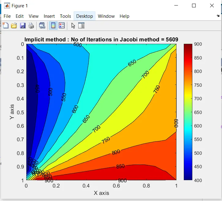
Figure 10 : Implicit method : jacobi method , convergence plot
1) jacobi method 2) Gauss seidel 3)Sucessive over relaxation
 Enter an option for the type of solver u want to use :
 1

CFL =

    0.5488

No of iterations in jacobi method =5609

time_taken =

    1.6437

>>
Figure 11 : No of iterations and time taken
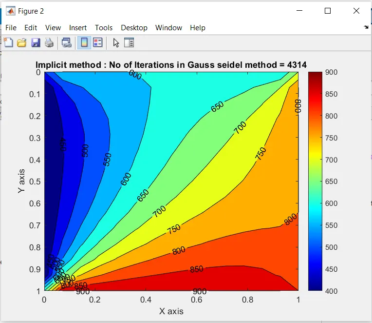
Figure 12 : Implicit method : Gauss-siedel method , convergence plot
1) jacobi method 2) Gauss seidel 3)Sucessive over relaxation
 Enter an option for the type of solver u want to use :
 2

CFL =

    0.5488

No of iterations in Gauss seiedel method =4314

time_taken =

    1.4684
Figure 13 : No of iterations and time taken
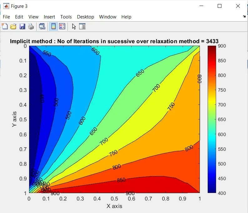
Figure 14 : Implicit method : Sucessive over relaxation method , convergence plot
1) jacobi method 2) Gauss seidel 3)Sucessive over relaxation
 Enter an option for the type of solver u want to use :
 3

CFL =

    0.5488

No of iterations in sucessive over relaxation method =3433

time_taken =

    1.6316
Figure 15 : No of iterations and time taken
RESULTS AND DISCUSSION :
1. We can see that the No of iterations are lower in steady state equation than the unsteady equation , this is because in the first case the the quation is only dependent to spatial co-ordinates where as in the later case the equation is dependent to time and spatial co-ordinates .
2. We can see that the explicit method seems to quiet simpler but its less accurate .
3. Transient solvers take a lot of computing time .
4. The no of iterations and time taken for the steady state and unsteady state respectively are lower for sucessive over relaxation method (iterative solver) then the other two solvers .
5. From the report we can say that the computing time is higher for the jacobi method and the no of iterations is also higher for the jacobi method and the iteration and computing time is lower for the sucessive over relaxation method , the oder of iterations is as follows :
Jacobi method > Gauss seiedel method > Sucessive over relaxation method .
.............................................................................END...........................................................