Solving the steady and unsteady 2D heat conduction problem

AIM:-

To perform transient and steady-state analysis of temperature evolution for a 2D domain with the given boundary conditions:

Top Boundary = 600 K

Bottom Boundary = 900 K

Left Boundary = 400 K

Right Boundary = 800 K

And to compare the explicit and implicit methods of Jacobi, Gauss-Seidel, and Successive Over-Relaxation (SOR) to solve the transient system.

THEORY:-

The governing equation for temperature evolution in a 2D domain is

`(d^2T)/dx^2+(d^2T)/dy^2= (1/alpha)*(dT)/dt`

*note that this is a partial differential equation (PDE)

where,

T - temperature (K)

t - time (s)

alpha - thermal diffusivity

x and y - the spatial coordinates in each of the 2 dimensions

For Steady State

`(d^2T)/dx^2+(d^2T)/dy^2=0`

This equation doesn't have the RHS term since it is steady-state and therefore temperature (T) doesn't vary with time (t).

This equation is of the elliptic type. The iterative methods will help calculate the equilibrium temperature based on the given boundary conditions.

The numerical solution can be obtained by the use of iterative techniques such as:

Jacobi method

`(T^(k)(i-1,j)-2*T^(k+1)(i,j)+T^(k)(i+1,j))/(dx^2)+(T^(k)(i,j-1)-2*T^(k+1)(i,j)+T^(k)(i,j+1))/(dy^2) = 0`

where,

the superscript k+1 represents the current iteration no. and k is the previous iteration.

dx and dy are the element lengths in the x and y dimensions respectively.

This method takes the values from the adjacent grid points in the previous iteration to calculate the T at the next iteration.

Gauss-Seidel method

`(T^(k+1)(i-1,j)-2*T^(k+1)(i,j)+T^(k)(i+1,j))/(dx^2)+(T^(k+1)(i,j-1)-2*T^(k+1)(i,j)+T^(k)(i,j+1))/(dy^2) = 0`

This method takes values from the current and previous iteration to calculate the value of T at the current iteration.

SOR method

`T^(k+1)(i,j) = (1-omega)*T^(k)(i,j)+(omega/2)*((dy^2/(dx^2+dy^2))*(T^(k+1)(i-1,j)+T^(k)(i+1,j))+(dx^2/(dx^2+dy^2))*(T^(k)(i,j+1)+T^(k+1)(i,j-1)))`

This method uses a relaxation factor in combination with the Gauss-Seidel method to iterate towards the solution.

In all of these methods, a tolerance value is set. This is used to check the difference between 2 consecutive iterations and if the difference between the temperatures in the domain in each is below the allotted tolerance value then it is understood that the system has iterated to the correct temperature values.

For Unsteady State

(d^2T)/dx^2+(d^2T)/dy^2= (1/alpha)*(dT)/dt

This is a parabolic equation.

Explicit method

This method uses the Forward Time Central Space (FTCS) scheme to evolve the temperature values at the grid points through each time step. This can be kept stable by satisfying the condition that the sum of the diffusion numbers (d_x and d_y) is less than or equal to 0.5.

`1/alpha*(T^(n+1)(i,j)-T^(n)(i,j))/dt= (T^(n)(i-1,j)-2*T^(n)(i,j)+T^(n)(i+1,j))/(dx^2)+(T^(n)(i,j-1)-2*T^(n)(i,j)+T^(n)(i,j+1))/(dy^2)`

here,

superscript n is previous time step and n+1 is current time step

This can be reduced to

`T^(n+1)(i,j) = T^(n)(i,j)*(1-2*d_x-2d_y)+d_x*(T^(n)(i-1,j)+T^(n)(i+1,j))+d_y*(T^(n)(i,j-1)+T^(n)(i,j+1))`

where

`d_x = (alpha*dt)/dx^2` - is the diffusion no. in the x dimension

`d_y = (alpha*dt)/dy^2` - is the diffusion no. in the y dimension

For stability

`d_x +d_y <= 0.5`

This method only requires temporal iteration/execution since each time you execute the formula you get the values for the next time step. The temporal iteration helps achieve the steady-state temperature by using a tolerance value.

Implicit methods

These methods use values from the current time step (n+1) to calculate the value of the other grid points in the current time step (n+1). The values from the current time step that are not known are assumed from the previous time step (n). The implicit system has unconditional stability, unlike the explicit methods, and is hence preferred.

`T^(n+1)(i,j) = (T^(n)(i,j))/(1+2*d_x+2*d_y)+d_x/(1+2*d_x+2*d_y)*(T^(n+1)(i-1,j)+T^(n+1)(i+1,j))+d_y/(1+2*d_x+2*d_y)*(T^(n+1)(i,j-1)+T^(n+1)(i,j+1))`

These methods however require iteration in the spatial domain since we do not have the values at all points in the current time step (n+1) initially, we need to take guess values which we take from the previous time step (n) and then iterate those values spatially using one of the Jacobi, Gauss-Seidel or SOR iteration methods to get the accurate temperature values at that time step (n+1) before moving to the next time step (n+2).

The Jacobi, Gauss-Seidel (GS), and SOR iteration methods will be implemented as shown in the steady-state case to execute the spatial iteration.

METHOD:-

For Steady State

The main code

• The code starts with the set up of the domain. The length of the domain in each dimension (L_x and L_y) and the number of nodes in each (n_x and n_y) are defined. The grid of points in the domain is created using the meshgrid function.
  
  
• The temperature (T) matrix is initialized and the boundary conditions are applied at the boundaries and the values at the corners are interpolated based on the boundary values. The initial guess value is applied at all of the interior points during the initialization of the T matrix, this is taken as the average of the temperatures at the boundaries.
• The menu function is used to give the user the option to select which iterative method is to be applied. The tolerance value is also inputted.
  
  
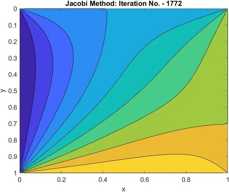
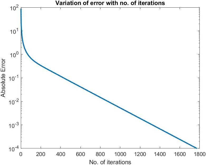
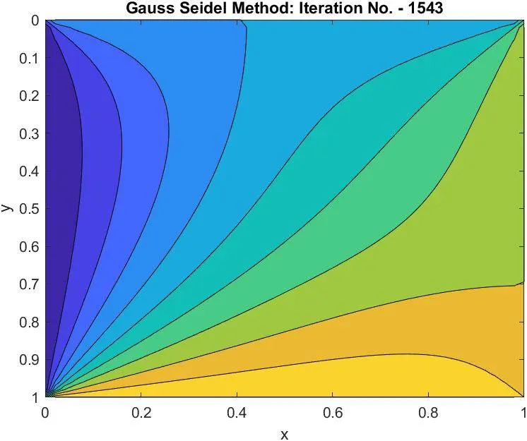
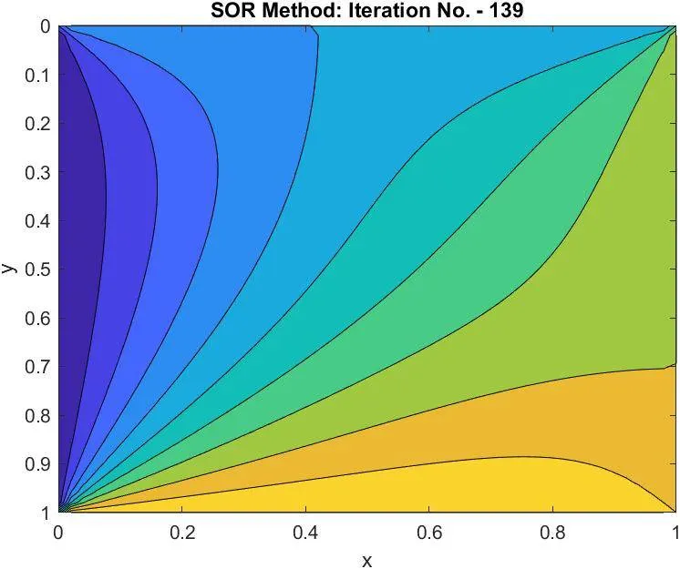
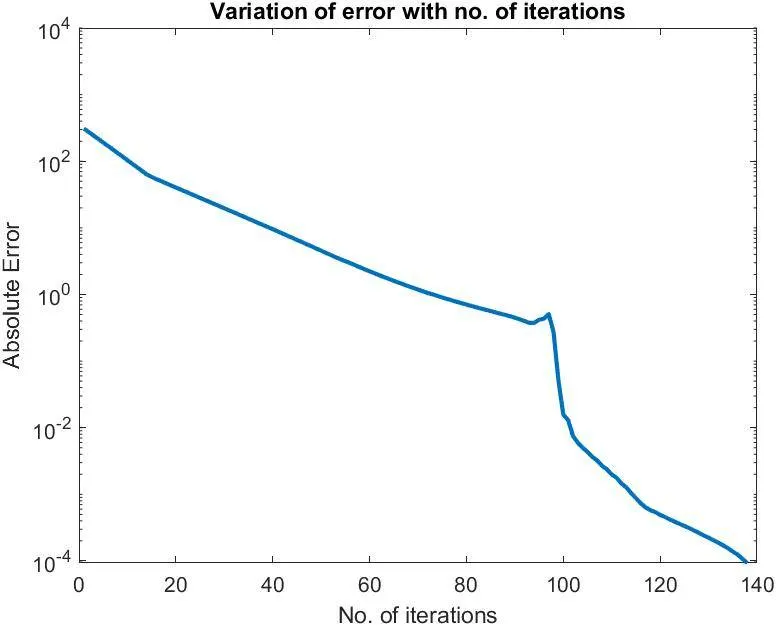
• if condition is used to run the different iterative methods (Jacobi, GS, or SOR) based on the user's choice. Each of the choices leads to a function that executes that particular iteration scheme, gives a final contour plot of the temperature in the domain and a plot showing the variation of error with the number of iterations.
  
  
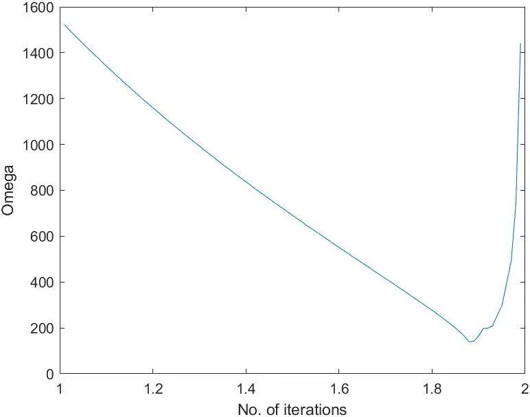
• For the SOR method, the optimum value of the relaxation factor (omega) is calculated by running the sor function for each value of omega between 1 and 2 and then the optimum value of omega (omega_opt) is used to run the sor function and plot the final temperature contour. The optimum value is obtained by checking for the value of omega that requires the least number of iterations to have the error fall below tolerance.
  
  

% Two-Dimensional Heat Conduction Solver
% d^2T/dx^2 + d^2T/dy^2 = 0
%Elliptic

clear all
close all
clc

%To input 
%Known information

L_x = 1; % Domain length in x dimension
L_y = 1; % Domain length in y dimension

n_x = 50; % No. of nodes in x dimension
n_y = 50; % No. of nodes in y dimension

dx = L_x/n_x; %Mesh Element size in x dimension
dy = L_y/n_y; %Mesh Element size in y dimension

x = linspace(0,L_x,n_x);
y = linspace(0,L_y,n_y);

[xx yy] = meshgrid(x,y);

%Boundary conditions

T_north = 600;
T_south = 900;
T_west = 400;
T_east = 800;

%Initializing the temperature matrix
T = zeros(n_x,n_y);

%Taking initial guess as sum of boundary values
T(:,:) = (T_east+T_west+T_south+T_north)/4;


%From the boundary conditions, we know that
T(1,:) = T_north;
T(n_y,:) = T_south;
T(:,1) = T_west;
T(:,n_x) = T_east;

%Taking average of boundary values at corners
T(1,1) = (T_north+T_west)/2;
T(n_y,1) = (T_south+T_west)/2;
T(1,n_x) = (T_north+T_east)/2;
T(n_y,n_x) = (T_south+T_east)/2;

%Creating the user menu
list = {'Jacobi method','Gauss Seidel method','SOR method'};
choice = menu('Choose the iterative method to be used',list)
iteration_solver = choice;

error = 9e9;

tolerance = 1e-4;

T_old = T;

if iteration_solver == 1
    %Jacobi method
    [T_jac,e,ctr,iter] = jacobi(T,n_x,n_y,dx,dy,tolerance);
    
    %To plot the final temperature distribution
    figure(1)
    surf(xx,yy,T_jac)
    xlabel('x')
    ylabel('y')
    zlabel('Temperature')
    title_text = sprintf('Jacobi Method: Iteration No. - %d',ctr);
    title(title_text)
    
    %To plot the variation of error with each iteration
    figure(3)
    plot(iter,e,'linewidth',2)
    xlabel('No. of iterations')
    ylabel('Absolute Error')
    title('Variation of error with no. of iterations')
end

if iteration_solver == 2

    %Gauss-Seidel method
    [T_gs,e,ctr,iter] = gauss_seidel(T,n_x,n_y,dx,dy,tolerance);
    
    %To plot the final temperature distribution
    figure(1)
    surf(xx,yy,T_gs)
    xlabel('x')
    ylabel('y')
    zlabel('Temperature')
    title_text = sprintf('Gauss Seidel Method: Iteration No. - %d',ctr);
    title(title_text)
    
    %To plot the variation of error with each iteration
    figure(3)
    plot(iter,e,'linewidth',2)
    xlabel('No. of iterations')
    ylabel('Absolute Error')
    title('Variation of error with no. of iterations')
end     

if iteration_solver == 3
    
    %To find the optimum value of omega
    omega_range = 0.01:0.01:1.3;

    for k = 1:length(omega_range)
        omega = omega_range(k);
        [~,~,ctr,~] = sor(T,n_x,n_y,dx,dy,tolerance,omega);
        iterations(k) = ctr;
        
    end

    opt = find(iterations == min(iterations));
    omega_opt = omega_range(opt);
    
    plot(omega_range,iterations)
    
    %Over-relaxation factor
    omega = omega_opt;
    %Successive Over-Relaxation (SOR) method

        [T_sor,e,ctr,iter] = sor(T,n_x,n_y,dx,dy,tolerance,omega);
    
    %To plot the final temperature distribution
    figure(1)
    surf(xx,yy,T_sor)
    xlabel('x')
    ylabel('y')
    zlabel('Temperature')
    title_text = sprintf('SOR Method: Iteration No. - %d',ctr);
    title(title_text)
    
    %To plot the variation of error with each iteration
    figure(3)
    plot(iter,e,'linewidth',2)
    xlabel('No. of iterations')
    ylabel('Absolute Error')
    title('Variation of error with no. of iterations')
end

Jacobi function

• The Jacobi function takes the input of the initial guess temperature (T), the no. of grid points in x and y (n_x and n_y), and the tolerance value to output the final/correct temperature values, the no. of iterations and the error values calculated at each iteration step.
  
  
• To ensure that the final temperature value with the error below tolerance is obtained, a while loop is used with the condition while error>tolerance. Within that loop, a for loop is run to apply the Jacobi discretized formula across all of the interior points (i.e, points not on the boundary). Also within the while loop, the error is calculated after the T has been calculated for all the points in a particular iteration by taking the difference between the T from the previous iteration and the T found in the current iteration. Also, a ctr variable is increased by 1 in each execution of the while loop to keep track of the number of iterations and the T from this iteration is stored in T_old since, in the next iteration of the while loop, it will be the value of T from the previous iteration and can be used to calculate the error.

%Jacobi Method
function [T_jac,e,ctr,iter] = jacobi(T,n_x,n_y,dx,dy,tolerance)

T_old = T;
T_jac = T;
ctr = 1;
error = 9e9;

    while (max(error)>tolerance)
            for j = 2:(n_y - 1)
                for i = 2:(n_x - 1)
                    T_jac(j,i) =  (1/2)*(((dy^2)/((dx^2)+(dy^2)))*(T_old(j-1,i)+T_old(j+1,i))+((dx^2)/((dx^2)+(dy^2)))*(T_old(j,i+1)+T_old(j,i-1))); 
                end
            end
        error = max(max(abs(T_old - T_jac)));
        iter(ctr) = ctr;
        e(ctr) = max(error);
        ctr = ctr+1;
        T_old = T_jac;
    end

end

Gauss-Seidel function

• This also runs similar to the Jacobi function except that the formula is changed to the GS formula.

%Gauss Seidel Method
function [T_gs,e,ctr,iter] = gauss_seidel(T,n_x,n_y,dx,dy,tolerance)

T_old = T;
T_gs = T;
ctr = 1;
error = 9e9;

    while (max(error)>tolerance)
            for j = 2:(n_y - 1)
                for i = 2:(n_x - 1)
                    T_gs(j,i) =  (1/2)*(((dy^2)/((dx^2)+(dy^2)))*(T_gs(j-1,i)+T_old(j+1,i))+((dx^2)/((dx^2)+(dy^2)))*(T_old(j,i+1)+T_gs(j,i-1))); 
                end
            end
        error = max(max(abs(T_old - T_gs)));
        iter(ctr) = ctr;
        e(ctr) = max(error);
        ctr = ctr+1;
        T_old = T_gs;
    end

end

Successive Over-Relaxation (SOR) function

• This also runs similar to the Jacobi function except that the formula is changed to the SOR formula.

%Successive Over Relaxation (SOR) Method
function [T_sor,e,ctr,iter] = sor(T,n_x,n_y,dx,dy,tolerance,omega)

T_old = T;
T_sor = T;
ctr = 1;
error = 9e9;
tic
    while (max(error)>tolerance)
            for j = 2:(n_y - 1)
                for i = 2:(n_x - 1)
                    T_sor(j,i) =  T_old(j,i)+(omega/2)*(((dy^2)/((dx^2)+(dy^2)))*(T_sor(j-1,i)+T_old(j+1,i))+((dx^2)/((dx^2)+(dy^2)))*(T_old(j,i+1)+T_sor(j,i-1))-2*T_old(j,i)); 
                end
            end
        error = max(max(abs(T_old - T_sor)));
        iter(ctr) = ctr;
        e(ctr) = max(error);
        ctr = ctr+1;
        T_old = T_sor;
        
    end

end

PLOTS:-

For Jacobi method

For Gauss-Seidel method

For the SOR method

OBSERVATIONS:-

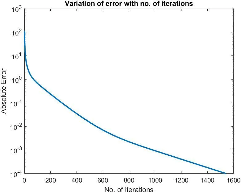
It can be observed that the no. of iterations required to arrive at the converged (error<tolerance) result is the least for SOR<Gauss-Seidel

The optimum relaxation factor for SOR is 1.88.

METHOD:-

For Unsteady State

The main code

• The code starts with the set up of the domain. The length of the domain in each dimension (L_x and L_y) and the number of nodes in each (n_x and n_y) are defined. The grid of points in the domain is created using the meshgrid function.
  
  
• The temperature (T) matrix is initialized and the boundary conditions are applied at the boundaries and the values at the corners are interpolated based on the boundary values. The initial guess value is applied at all of the interior points during the initialization of the T matrix, this is taken as the average of the temperatures at the boundaries.
  
  
• The menu function is used to give the user the option to select which iterative method is to be applied. The tolerance value is also inputted.
  
  
• if condition is used to run the different iterative methods (Explicit, Jacobi, GS, or SOR) based on the user's choice. Each of the choices leads to a function within the main code that executes that particular iteration scheme, gives the contour plots of the temperature in the domain for each time step and these plots are used to create an animation.
  
  
• For the Explicit scheme portion
  
  • A while loop is used with the condition while error>tolerance. Within that loop, 2 for loops are run to apply the Jacobi discretized formula across all of the interior points (i.e, points not on the boundary). Also within the while loop, the error is calculated after the T has been calculated for all the points in a particular iteration by taking the difference between the T from the previous iteration and the T found in the current iteration. The contour plots are plotted for each time step and the plots are stored in a matrix M in order to create the animation later. Also, a ctr variable is increased by 1 in each execution of the while loop to keep track of the number of iterations and the T from this iteration is stored in T_old since, in the next iteration of the while loop, it will be the value of T from the previous iteration and can be used to calculate the error.
    
    
• For the Jacobi implicit portion
  • Here there are 2 while loops to run the temporal and spatial iterations both of which check for error between consecutive time steps and spatial iterations respectively. Within the second spatial while loop there are 2 for loops that ensure all of the interior points are covered and then the error between consecutive spatial iterations is calculated and the iteration counter (iter) is incremented and the current T values are stored in T_old since they will be previous iteration values in the next spatial iteration. Outside of the spatial while loop but still within the temporal while loop the error between consecutive time steps are checked and the time step counter (t_step) is incremented and the T values are stored in T_prev_dt for the next time step. Also, the tic-toc function is used to calculate the time required to run the scheme.
• For the Gauss-Seidel implicit portion
  • This is similar to the above with just the GS formula implemented.
    
    
• For the Gauss-Seidel implicit portion
  • This is similar to the above with just the SOR formula implemented.
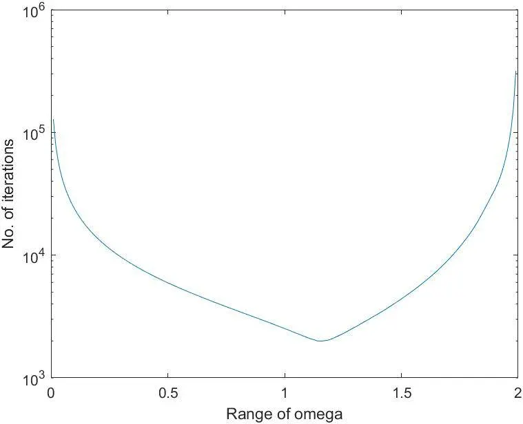
  • For the SOR method, the optimum value of the relaxation factor (omega) is calculated by running the imp_sor function for each value of omega between 1 and 2 and then the optimum value of omega (omega_opt) is used to run the imp_sor function in the main code and plot the temperature contours. The optimum value is obtained by checking for the value of omega that requires the least number of iterations to have the error fall below tolerance.

% Unsteady State Two-Dimensional Heat Conduction Solver
% d^2T/dx^2 + d^2T/dy^2 = (1/alpha)*(dT/dt)
%Parabolic Equation

clear all
close all
clc

%To input 
%Known information

L_x = 1; % Domain length in x dimension
L_y = 1; % Domain length in y dimension

n_x = 20; % No. of nodes in x dimension
n_y = n_x; % No. of nodes in y dimension

dx = L_x/n_x; %Mesh Element size in x dimension
dy = L_y/n_y; %Mesh Element size in y dimension

x = linspace(0,L_x,n_x);
y = linspace(0,L_y,n_y);

[xx yy] = meshgrid(x,y);

%Boundary conditions

T_north = 600;
T_south = 900;
T_west = 400;
T_east = 800;

%Initializing the temperature matrix
T = zeros(n_x,n_y);

%Taking initial guess as sum of boundary values
T(:,:) = (T_east+T_west+T_south+T_north)/4;

%From the boundary conditions, we know that
T(1,:) = T_north;
T(n_y,:) = T_south;
T(:,1) = T_west;
T(:,n_x) = T_east;

%Taking average of boundary values at corners
T(1,1) = (T_north+T_west)/2;
T(n_y,1) = (T_south+T_west)/2;
T(1,n_x) = (T_north+T_east)/2;
T(n_y,n_x) = (T_south+T_east)/2;

%Diffusion No.
dt = 2.5e-4;
alpha = 1.5;
d_x = (alpha*dt)/(dx^2);
d_y = (alpha*dt)/(dy^2);

t_end = 10;

list = {'Explicit Method','Implicit Jacobi method','Implicit Gauss Seidel method','Implicit SOR method'};
choice = menu('Choose the iterative method to be used',list)
iteration_solver = choice;



error_iter = 9e9;
error_time = 9e9;
tolerance = 1e-4;

T_old = T;
T_prev_dt = T;

iter = 1;
t_step = 1;
ctr = 1;

if iteration_solver == 1
    tic
   
    %Explicit Scheme

        while(error_time>tolerance)
            for j = 2:(n_y - 1)
                for i = 2:(n_x - 1)
                    T(j,i) =  ((1- 2*d_x - 2*d_y)*T_prev_dt(j,i)+d_x*(T_prev_dt(j-1,i)+T_prev_dt(j+1,i))+d_y*(T_prev_dt(j,i-1)+T_prev_dt(j,i+1)));
                end
            end
            error_time = max(max(abs(T-T_prev_dt)));
            T_prev_dt = T;
            contourf(xx,yy,T)
            axis ij
            xlabel('x')
            ylabel('y')
            zlabel('Temperature')
            title_text = sprintf('Explicit Method: Time - %g, Time Step - %d',ctr*dt,ctr);
            title(title_text)
            pause(0.3)
            M(ctr) = getframe(gcf);
            ctr = ctr+1;
        end
        exp_time = toc;
        
%For Implicit Jacobi scheme (Laasonen method)

elseif iteration_solver == 2
   tic
   while (error_time>tolerance)
       error_iter = 9e9;
       while (error_iter>tolerance)
           for j = 2:(n_y - 1)
               for i = 2:(n_x - 1)
                    T(j,i) =  (1/(1+ 2*d_x + 2*d_y))*T_prev_dt(j,i)+(d_x/(1+ 2*d_x + 2*d_y))*(T_old(j-1,i)+T_old(j+1,i))+(d_y/(1+ 2*d_x + 2*d_y))*(T_old(j,i-1)+T_old(j,i+1));
               end
           end
       error_iter = max(max(abs(T_old - T)));
       T_old = T;
       iter = iter+1;
       end
       error_time = max(max(abs(T_prev_dt - T)));
       T_prev_dt = T;
       contourf(xx,yy,T)
       axis ij
       xlabel('x')
       ylabel('y')
       zlabel('Temperature')
       title_text = sprintf('Jacobi Method (Implicit): Time - %g s: Steps - %d',t_step*dt,t_step);
       title(title_text)
       pause(0.3)
       M(t_step) = getframe(gcf);
       t_step = t_step + 1;
   end
   imp_jac_time = toc; 
   
   %For Implicit Gauss Seidel method
elseif iteration_solver == 3
    tic
    while (error_time>tolerance)
       error_iter = 9e9;
       while (error_iter>tolerance)
           for j = 2:(n_y - 1)
               for i = 2:(n_x - 1)
                    T(j,i) =  (1/(1+ 2*d_x + 2*d_y))*T_prev_dt(j,i)+(d_x/(1+ 2*d_x + 2*d_y))*(T(j-1,i)+T(j+1,i))+(d_y/(1+ 2*d_x + 2*d_y))*(T(j,i-1)+T(j,i+1));
               end
           end
       error_iter = max(max(abs(T_old - T)));
       T_old = T;
       iter = iter+1;
       end
       error_time = max(max(abs(T_prev_dt - T)));
       T_prev_dt = T;
       contourf(xx,yy,T)
       axis ij
       xlabel('x')
       ylabel('y')
       zlabel('Temperature')
       title_text = sprintf('Gauss Seidel Method (Implicit): Time - %g s: Steps - %d',t_step*dt,t_step);
       title(title_text)
       pause(0.3)
       M(t_step) = getframe(gcf);
       t_step = t_step + 1;
    end
    imp_gs_time = toc;
%For Implicit SOR method

elseif iteration_solver == 4
    %To find the optimum value of omega
    omega_range = 0.01:0.01:1.99;

    for k = 1:length(omega_range)
        omega = omega_range(k);
        [~,iter,t_step] = imp_sor(T,n_x,n_y,d_x,d_y,tolerance,omega);
        iterations(k,1) = iter;
        iterations(k,2) = t_step;
        
    end

    opt = find(iterations == min(iterations(:,1)));
    omega_opt = max(omega_range(opt));
    
    figure(1)
    semilogy(omega_range,iterations(:,1))
    xlabel('Range of omega')
    ylabel('No. of iterations')
    
    iter_main = 1;
    t_step_main = 1;
    
    tic
    omega = omega_opt;
    while (error_time>tolerance)
       error_iter = 9e9;
       while (error_iter>tolerance)
           for j = 2:(n_y - 1)
               for i = 2:(n_x - 1)
                    T(j,i) =  T_old(j,i) + omega*((1/(1+ 2*d_x + 2*d_y))*T_prev_dt(j,i)+(d_x/(1+ 2*d_x + 2*d_y))*(T(j-1,i)+T(j+1,i))+(d_y/(1+ 2*d_x + 2*d_y))*(T(j,i-1)+T(j,i+1))-T_old(j,i));
               end
           end
       error_iter = max(max(abs(T_old - T)));
       T_old = T;
       iter_main = iter_main+1;
       end
       error_time = max(max(abs(T_prev_dt - T)));
       T_prev_dt = T;
       figure(2)
       contourf(xx,yy,T)
       axis ij
       xlabel('x')
       ylabel('y')
       zlabel('Temperature')
       title_text = sprintf('SOR Method (Implicit): Time - %g s: Steps - %d',t_step_main*dt,t_step_main);
       title(title_text)
       pause(0.3)
       M(t_step_main) = getframe(gcf);
       t_step_main = t_step_main + 1;
    end
   imp_sor_time = toc;
end

% To create the animation videofile

movie(M)
if choice == 1
    filename = sprintf('Explicit_animation.avi');
elseif choice == 2
    filename = sprintf('Jacobi_implicit_animation.avi');
elseif choice == 3
    filename = sprintf('GS_implicit_animation.avi');
elseif choice == 4
    filename = sprintf('SOR_implicit_animation.avi');
end
videofile = VideoWriter(filename,'Uncompressed AVI');
open(videofile)
writeVideo(videofile,M)
close(videofile)

%To display the time required
if choice == 1
    time = sprintf('The time taken by Explicit Method is %d s',exp_time);
elseif choice == 2
    time = sprintf('The time taken by Implicit Jacobi Method is %d s',imp_jac_time);
elseif choice == 3
    time = sprintf('The time taken by Implicit Gauss Seidel Method is %d s',imp_gs_time);
elseif choice == 4
    time = sprintf('The time taken by Implicit SOR Method is %d s',imp_sor_time);
end

disp(time);

The Implicit Successive Over-Relaxation (SOR) function

%Implicit SOR method
function [T_sor,iter,t_step] = imp_sor(T,n_x,n_y,d_x,d_y,tolerance,omega)

T_sor = T;
T_prev_dt = T;
T_old = T;
iter = 1;
error_time = 9e9;
error_iter = 9e9;
t_step = 1;


while (error_time>tolerance)
   error_iter = 9e9;
   while (error_iter>tolerance)
       for j = 2:(n_y - 1)
           for i = 2:(n_x - 1)
                T_sor(j,i) =  T_old(j,i) + omega*((1/(1+ 2*d_x + 2*d_y))*T_prev_dt(j,i)+(d_x/(1+ 2*d_x + 2*d_y))*(T_sor(j-1,i)+T_sor(j+1,i))+(d_y/(1+ 2*d_x + 2*d_y))*(T_sor(j,i-1)+T_sor(j,i+1))-T_old(j,i));
           end
       end
   error_iter = max(max(abs(T_old - T_sor)));
   T_old = T_sor;
   iter = iter+1;
   end
   error_time = max(max(abs(T_prev_dt - T_sor)));
   t_step = t_step + 1;
   T_prev_dt = T_sor;
end

end

PLOTS:-

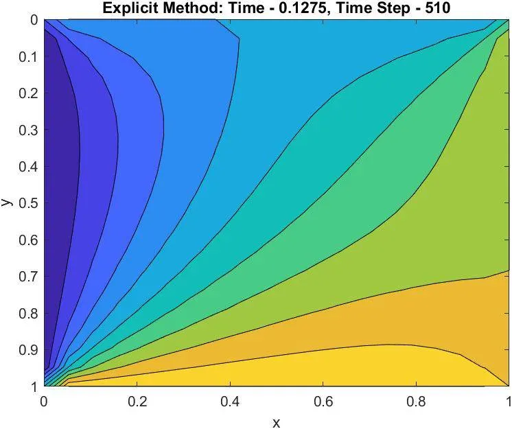
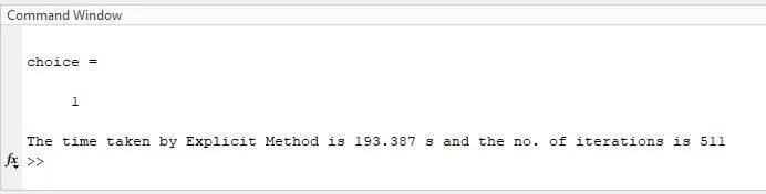
For Explicit method

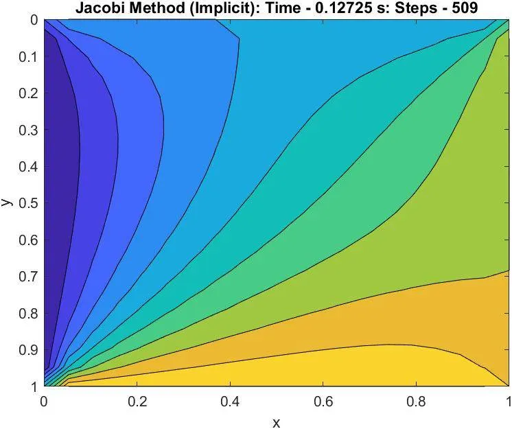
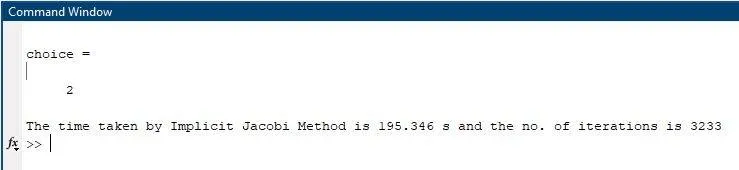
For Implicit Jacobi method

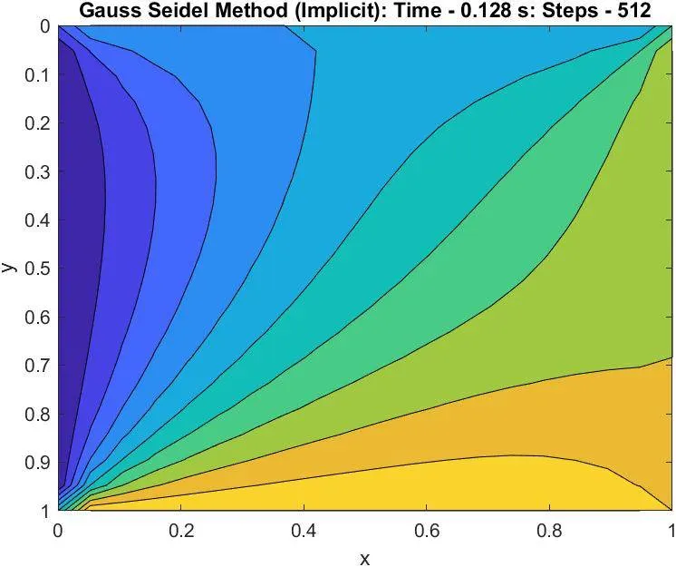
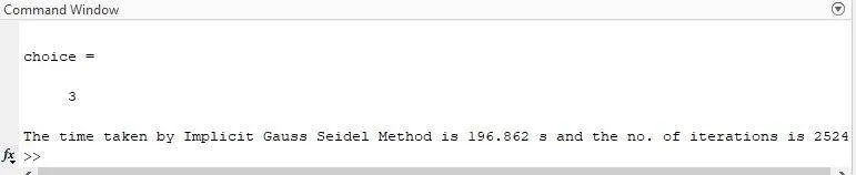
For Implicit Gauss-Seidel method

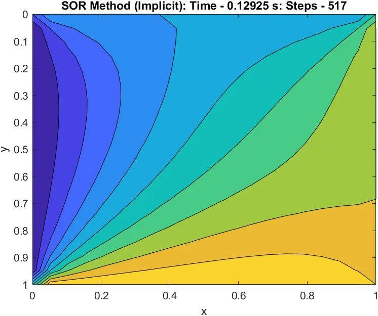
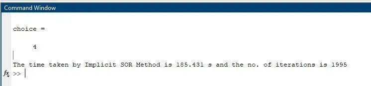
For Implicit SOR method

OBSERVATIONS:-

It can be observed that the no. of iterations required to arrive at the steady-state solution is Explicit<SOR<Gauss-Seidel<Jacobi.

The optimum relaxation factor for SOR is 1.16.

Link to the animations are below

Unsteady state - Explicit - Jacobi - Gauss-Seidel - SOR