Taylor table method and MATLAB code

AIM:-

To calculate the second-order derivative of the following function:-

`f(x) = exp(x)*cos(x)`

using central difference, skewed forward difference, and skewed backward difference schemes of fourth-order accuracy.

THEORY:-

The formula for the discretized derivative in each of the schemes is obtained using the Taylor Table method.

For Central Difference

	f(x)	f'(x)dx	f''(x)dx^2	f'''(x)dx^3	f''''(x)dx^4	f'''''(x)dx^5	f''''''(x)dx^6
a*f(x-2dx)	a	-2a	2a	-4a/3	2a/3	-4a/15	4a/45
b*f(x-dx)	b	-b	b/2	-b/6	b/24	-b/120	b/720
c*f(x)	c	0	0	0	0	0	0
d*f(x+dx)	d	d	d/2	d/6	d/24	d/120	d/720
e*f(x+2dx)	e	2e	2e	4e/3	2e/3	4e/15	4e/45
f''(x)	0	0	1/dx^2	0	0	0	0

where, `f''(x) = (a*f_(i-2)+b*f_(i-1)+c*f_i+d*f_(i+1)+e*f_(i+2))/dx^2`+ O(dx^4)

For Forward Differencing (Skewed)

	f(x)	f'(x)dx	f''(x)dx^2	f'''(x)dx^3	f''''(x)dx^4	f'''''(x)dx^5	f''''''(x)dx^6
a*f(x)	a	0	0	0	0	0	0
b*f(x+dx)	b	b	b/2	b/6	b/24	b/120	b/720
c*f(x+2dx)	c	2c	2c	4c/3	2c/3	4c/15	4c/45
d*f(x+3dx)	d	3d	9d/2	9d/2	27d/8	81d/40	81d/80
e*f(x+4dx)	e	4e	8e	32e/3	32e/3	128e/15	216e/45
g*f(x+5dx)	g	5g	25g/2	125g/6	625g/24	625g/24	3125g/144
f''(x)	0	0	1/dx^2	0	0	0	0

here, `f''(x) = (a*f_(i)+b*f_(i+1)+c*f_(i+2)+d*f_(i+3)+e*f_(i+4)+g*f_(i+5))/dx^2``+ O(dx^4)

For Backward Differencing (Skewed)

	f(x)	f'(x)dx	f''(x)dx^2	f'''(x)dx^3	f''''(x)dx^4	f'''''(x)dx^5	f''''''(x)dx^6
a*f(x)	a	0	0	0	0	0	0
b*f(x-dx)	b	-b	b/2	-b/6	b/24	-b/120	b/720
c*f(x-2dx)	c	-2c	2c	-4c/3	2c/3	-4c/15	4c/45
d*f(x-3dx)	d	-3d	9d/2	-9d/2	27d/8	-81d/40	81d/80
e*f(x-4dx)	e	-4e	8e	-32e/3	32e/3	-128e/15	216e/45
g*f(x-5dx)	g	-5g	25g/2	-125g/6	625g/24	-625g/24	3125g/144
f''(x)	0	0	1/dx^2	0	0	0	0

here, `f''(x) = (a*f_(i)+b*f_(i-1)+c*f_(i-2)+d*f_(i-3)+e*f_(i-4)+g*f_(i-5))/dx^2`+ O(dx^4)

These columns in these tables are added up to get equations and the system of equations is solved to obtain the values of the coefficients and thereby obtain the discretized formula.

Check Order of Accuracy

To check the order of accuracy of the method, the values of the coefficients obtained must be substituted into the equations that were not utilized in the calculation of the coefficients.

The order of power of the dx term remaining is the order of accuracy of the scheme.

For skewed FD:-

RHS = (b/720 + 4*c/45 + 81*d/80 + 216*e/45 + 3125*g/144)*dx^6

From solving we obtain that,

a = 15/4*dx^2; b = -77/6*dx^2; c = 107/6*dx^2; d = -13/dx^2; e = 61/12*dx^2; g = -5/6*dx^2;

Substituting into the equation, we get

RHS = -5.279*dx^4

Therefore, the order of accuracy is 4.

Similarly, for BD the order of accuracy is 4.

This proves that the thumb rule in HINT(ii) is correct.

METHOD:-

The fourth_order_coeffs function (coefficient function)

• This function is used to obtain the value of the coefficients by solving the system of equations using matrix inversion using the linsolve command.
  
  
• The function takes in the order of accuracy and solves the system of equations whose A and B matrices have been manually inputted using the data obtained from the Taylor Table.
  
  
• The function outputs the coefficient values for each scheme in respective columns of the coeffs matrix.

function [coeffs] = fourth_order_coeffs(oa)

if oa == 4
    A_CD4 = [1 1 1 1 1;-2 -1 0 1 2;2 1/2 0 1/2 2;-4/3 -1/6 0 1/6 4/3;2/3 1/24 0 1/24 2/3];

    B_CD = [0; 0; 1; 0; 0];

    B = [0; 0; 1; 0; 0; 0];

    A_FD4 = [1 1 1 1 1 1;0 1 2 3 4 5;0 1/2 2 9/2 8 25/2;0 1/6 4/3 9/2 32/3 125/6;0 1/24 2/3 27/8 32/3 625/24;0 1/120 4/15 81/40 128/15 625/24];

    A_BD4 = [1 1 1 1 1 1;0 -1 -2 -3 -4 -5;0 1/2 2 9/2 8 25/2;0 -1/6 -4/3 -9/2 -32/3 -125/6;0 1/24 2/3 27/8 32/3 625/24;0 -1/120 -4/15 -81/40 -128/15 -625/24];

    X_CD = linsolve(A_CD4,B_CD);
    X_FD = linsolve(A_FD4,B);
    X_BD = linsolve(A_BD4,B);

    coeffs(1:length(X_CD),1) = X_CD;
    coeffs(1:length(X_FD),2) = X_FD;
    coeffs(1:length(X_BD),3) = X_BD;
end
end

The numeric_disc_2ndorder function (error function)

• This function takes the values of x and the mesh element size (dx) and outputs the absolute error with respect to the analytically calculated derivative values. The error values are outputted in the form of an error matrix with each row corresponding to the error from each of the schemes.
  
  
• First, the analytic derivative is calculated, and then the central, forward (skewed) and backward (skewed) are calculated based on the coefficients calculated in the coeffs function. The function is called here to access the coefficient values and utilized in their respective formulas.

function [error] = numeric_disc_2ndorder(x,dx)

%Function f(x) = exp(x)*cos(x)
%Analytic Second-Order Derivative
%f''(x) = -2*exp(x)*sin(x)

anal_derivativ = -2*exp(x)*sin(x);

%Numerical Derivative

%Calling the function to obtain the coefficients for the discretized
%formulas
oa = 4;

[coeffs] = fourth_order_coeffs(oa);

%Central Difference (4th Order Accuracy)

num_deriv_cd_4 = (coeffs(1,1)*(exp(x-(2*dx))*cos(x-(2*dx)))+coeffs(2,1)*(exp(x-dx)*cos(x-dx))+coeffs(3,1)*(exp(x)*cos(x))+coeffs(4,1)*(exp(x+dx)*cos(x+dx))+coeffs(5,1)*(exp(x+(2*dx))*cos(x+(2*dx))))/(dx^2);

order_4_error_cd = abs(num_deriv_cd_4 - anal_derivativ);


%Forward Difference (Skewed)(4th Order Accuracy)

num_deriv_fd_4 = (coeffs(1,2)*(exp(x)*cos(x))+coeffs(2,2)*(exp(x+dx)*cos(x+dx))+coeffs(3,2)*(exp(x+(2*dx))*cos(x+(2*dx)))+coeffs(4,2)*(exp(x+(3*dx))*cos(x+(3*dx)))+coeffs(5,2)*(exp(x+(4*dx))*cos(x+(4*dx)))+coeffs(6,2)*(exp(x+(5*dx))*cos(x+(5*dx))))/(dx^2);

order_4_error_fd = abs(num_deriv_fd_4 -anal_derivativ);


%Backward Difference (Skewed)(4th Order Accuracy)

num_deriv_bd_4 = (coeffs(1,3)*(exp(x)*cos(x))+coeffs(2,3)*(exp(x-dx)*cos(x-dx))+coeffs(3,3)*(exp(x-2*dx)*cos(x-2*dx))+coeffs(4,3)*(exp(x-3*dx)*cos(x-3*dx))+coeffs(5,3)*(exp(x-4*dx)*cos(x-4*dx))+coeffs(6,3)*(exp(x-5*dx)*cos(x-5*dx)))/(dx^2);

order_4_error_bd = abs(num_deriv_bd_4 -anal_derivativ);


error(1) = order_4_error_cd;
error(2) = order_4_error_fd;
error(3) = order_4_error_bd;

end

The main code

• This starts with the input of the known values of x and the range of dx values (which are created using the linspace command).
  
  
• A for loop is created within which the error function is called and the error values obtained are sorted into seperate vectors for each of the schemes.
  
  
• The error values are then plotted in a log-log plot using the loglog command.
  

clear all
close all
clc

x = pi/3;
dx = linspace(pi/400,pi/20,20);

for i = 1:length(dx)

    error = numeric_disc_2ndorder(x,dx(i));
    CD4_error(i) = error(1);
    FD4_error(i) = error(2);
    BD4_error(i) = error(3);
    
end


loglog(dx,CD4_error,'linewidth',2,'color','b');
hold on
loglog(dx,FD4_error,'linewidth',2,'color','r');
hold on
loglog(dx,BD4_error,'linewidth',2,'color','g');
xlabel('log(Element Size)')
ylabel('log(Error)')
title('Comparing Error between the Schemes')
legend('CD-4 error','FD-4 (skewed) error','BD-4 (skewed) error')

PLOT:-

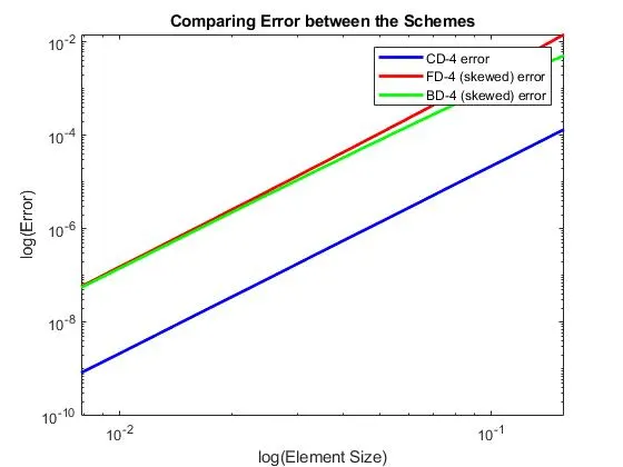
This plot shows that the CD-4 scheme has much lower error than the FD and BD skewed schemes.

It also indicates that the skewed FD and BD schemes have very similar errors.

Reason to use a skewed FD/BD scheme instead of CD

The skewed FD/BD schemes are more useful than a CD scheme along the edges of the mesh where there are only points to the left or right side of the point under consideration (i). So in these situations, the C formula cannot be applied as they require value from 2 points on the left and right of i. Therefore, in spite of the greater error in the skewed FD/BD schemes, they need to be used in place of the CD scheme.