Week 11 - Simulation of Flow through a pipe in OpenFoam
AIM:-
To simulate laminar-incompressible flow through a pipe using OpenFOAM using axisymmetric wedge boundary condition and MATLAB and validate with results obtained from Hagen-Poiseulle equation for fully developed flow.
MATLAB is used to automate the generation of the blockMeshDict file taking inputs like pipe diameter, Reynold's No., wedge angle, etc.
THEORY:-
Hagen-Poiseulle equation
This is a physical law that gives the pressure-drop in an incompressible and Newtonian fluid in laminar flow flowing through a cylindrical pipe of constant cross-section.
`trianglep=(32*mu*V_(avg)*L)/D^2`
where,
`trianglep`- pressure drop
`mu`- Dynamic viscosity
`V_(avg)`- average velocity
`L`- length of pipe
`D`- pipe diameter
Entry Length
However, this equation doesn't hold close to the pipe entrance and this is because the flow at the entrance of the pipe is not laminar. The flow is initially turbulent and after a certain length of pipe called the entry length of the pipe, the flow develops into laminar flow.
This is because the equation assumes a no-slip condition at the walls of the pipe, which causes the fluid particles in contact with the walls to come to a complete stop. This causes the fluid particles in adjacent layers to slow down as well due to viscous effects. To compensate for this the fluid at the center of the pipe will have greater velocity and this leads to the formation of a velocity gradient across the cross-section of the pipe. The region where the fluid particles are affected by viscous shear effects is called the velocity boundary layer.
This velocity boundary layer will grow as the flow continues along the pipe as the viscosity effects start to reach the center of the pipe and eventually the boundary layers from the top and bottom walls of the pipe will meet at the center and then the flow becomes fully developed and the velocity becomes constant. This is called the fully developed region.
So the flow along the pipe can be divided into 2 regions
- The region where the viscous effects and velocity changes are significant is called the hydrodynamic entrance region.
- The region where the viscous effects are insignificant and the velocity profile remains constant is the fully developed region.
The empirical formula for the hydrodynamic entry length is
`L_(entry) = 0.06*Re*D`
Beyond this length of the pipe, the flow becomes fully developed.
The shear stress for Newtonian (viscous) fluids is a function of the strain rate and the formula is
`tau = mu(du)/dy`
where (du)/dy is the strain rate
During laminar pipe flow,
The shear stress (tau) is maximum at the entrance due to the steeper velocity gradient and this reduces with the increasing thickness of the boundary layer. Once the flow becomes fully developed, the shear stress maintains a constant value.
Given Data
Working fluid is water
Reynold's No. (Re) = 2100
Assumptions
Wedge Angle = `2^circ`
Diameter (D) = 0.02 m
Temperature - `25 ^circC`
`implies`Density = 997.05 kg/m^3
Dynamic Viscosity (`mu`) = `8.9xx10^-4`Pa.s
Calculations
From the formula for Reynold's No. (Re)
`Re = (rhoxxVxxD)/mu`
`implies V = V_(avg) = (Rexxmu)/(rhoxxD)`
`implies V=V_(avg)=0.0937 m/s`
By Entry length empirical formula
`L_(entry) =`2.52 m
`therefore`Assume L = 3 m
By Hagen-Poiseulle equation
`trianglep`= 20.02 Pa
Kinematic Pressure drop (`trianglep_k) = (trianglep)/rho=`0.0201
METHOD:-
To generate the blockMeshDict file using MATLAB
- The code starts with defining the input parameters like wedge angle, pipe diameter, Reynold's No. (Re), density, dynamic viscosity, and the number of elements in each dimension.
- Then the values of velocity and pressure drop are calculated based on the Hagen-Poiseulle law.
- Then the vertices for the wedge block are defined.
- The rest of the code uses the fprintf command to develop the blockMeshDict code in the appropriate format while taking inputs from the calculated values.
- The wedge boundary condition is used for the sides of the wedge that would be in contact with the rest of the cylinder. This gives the axisymmetric cylinder effect as long as the wedge angle is `<=5^circ`
clear all
close all
clc
%To create the blockMeshDict file for OpenFOAM
%To create the section of the pipe
%Inputs
wedge_angle = 2;
D = 0.02; %Diameter
R = D/2; %Radius of pipe
half_angle = wedge_angle/2;
Re = 2100; %Reynold's No.
%Assuming fluid is water @ 25 C
rho = 997.05; %Density in kg/m^3
nu = 8.9*10^(-4); %Dynamic viscosity in Pa.s
%Defining No. of elements
n_z = 50; %No. of elements along the length of pipe (z direction)
n_x = 100; %No. of elements along radial direction (x direction)
n_y = 1; %No. of elements across the wedge face (y direction)
%Defining grading ratios
g_x = 1;
g_y = 1;
g_z = 0.2;
L_entry = 0.06*Re*D; %Entry length for laminar flow empirical formmula
L = round(L_entry,0); %Length of pipe
y = R*sind(half_angle);
x = R*cosd(half_angle);
%By definition Re = rho*v*D/mu
v = (Re*nu)/(rho*D);%Inlet velocity
%According to Hagen-Poiseulle law
v_avg = v;
v_max = 2*v_avg;
delta_p = (32*nu*L*v_avg)/(D^2); % Pressure drop
delta_p_k = delta_p/rho; %Kinematic pressure drop (due to icoFoam solver)
Q = pi*(R^2)*v_avg; %Flow Rate
disp(delta_p_k);
f1 = fopen('blockMeshDict_f','w');
%Creating the header of the blockMeshDict file
fprintf(f1,'%s \n', '/*--------------------------------*- C++ -*----------------------------------*\');
fprintf(f1,' ========= | \n');
fprintf(f1,' \\ / F ield | OpenFOAM: The Open Source CFD Toolbox \n');
fprintf(f1,' \\ / O peration | Website: https://openfoam.org \n');
fprintf(f1,' \\ / A nd | Version: 8 \n')
fprintf(f1,' \\/ M anipulation | \n')
fprintf(f1,'%s \n', '\*---------------------------------------------------------------------------*/');
fprintf(f1,'FoamFile \n');
fprintf(f1,'{ \n');
fprintf(f1,' version 2.0; \n');
fprintf(f1,' format ascii; \n');
fprintf(f1,' class dictionary; \n');
fprintf(f1,' object blockMeshDict; \n');
fprintf(f1,'} \n');
fprintf(f1,'%s \n', '// * * * * * * * * * * * * * * * * * * * * * * * * * * * * * * * * * * * * * //');
fprintf(f1,'\n');
fprintf(f1,'convertToMeters 1;');
fprintf(f1,'\n');
fprintf(f1,'vertices \n');
fprintf(f1,'( \n');
%To create the vertices for the wedge
%Defining the points
p0 = [0 0 0];
p1 = [x y 0];
p2 = [x y L];
p3 = [0 0 L];
p4 = [x -y 0];
p5 = [x -y L];
vertices = [p0;p1;p2;p3;p4;p5];
%To print them in the blockMesh file
for i = 1:length(vertices)
fprintf(f1,' (%d %d %d) // point %d \n',vertices(i,1),vertices(i,2),vertices(i,3),i-1);
end
fprintf(f1,'\n); \n \n');
%To define the blocks
fprintf(f1,'blocks \n');
fprintf(f1,'( \n');
fprintf(f1,' hex (0 4 1 0 3 5 2 3) (%d %d %d) simpleGrading (%d %d %d) \n',n_x,n_y,n_z,g_x,g_y,g_z);
fprintf(f1,'\n); \n \n');
%To define the edges
fprintf(f1,'edges \n');
fprintf(f1,'( \n');
fprintf(f1,' arc 1 4 (%d 0 0) \n',R);
fprintf(f1,' arc 2 5 (%d 0 %d) \n',R,L);
fprintf(f1,'\n); \n \n');
%To define the boundaries
fprintf(f1,'boundary \n');
fprintf(f1,'( \n');
%Inlet
fprintf(f1,' Inlet\n {\n');
fprintf(f1,' type patch;\n');
fprintf(f1,' faces\n');
fprintf(f1,' (\n');
fprintf(f1,' (0 4 1 0)\n');
fprintf(f1,' );\n');
fprintf(f1,' }\n');
%Outlet
fprintf(f1,' Outlet\n {\n');
fprintf(f1,' type patch;\n');
fprintf(f1,' faces\n');
fprintf(f1,' (\n');
fprintf(f1,' (3 2 5 3)\n');
fprintf(f1,' );\n');
fprintf(f1,' }\n');
%Axis
fprintf(f1,' Axis\n {\n');
fprintf(f1,' type empty;\n');
fprintf(f1,' faces\n');
fprintf(f1,' (\n');
fprintf(f1,' (0 3 3 0)\n');
fprintf(f1,' );\n');
fprintf(f1,' }\n');
%Wall
fprintf(f1,' Wall\n {\n');
fprintf(f1,' type wall;\n');
fprintf(f1,' faces\n');
fprintf(f1,' (\n');
fprintf(f1,' (4 5 2 1)\n');
fprintf(f1,' );\n');
fprintf(f1,' }\n');
%Wedge Sides_Left
fprintf(f1,' Wedge_Side_Left\n {\n');
fprintf(f1,' type wedge;\n');
fprintf(f1,' faces\n');
fprintf(f1,' (\n');
fprintf(f1,' (0 1 2 3)\n');
fprintf(f1,' );\n');
fprintf(f1,' }\n');
%Wedge Sides_Right
fprintf(f1,' Wedge_Side_Right\n {\n');
fprintf(f1,' type wedge;\n');
fprintf(f1,' faces\n');
fprintf(f1,' (\n');
fprintf(f1,' (0 3 5 4)\n');
fprintf(f1,' );\n');
fprintf(f1,' }\n');
fprintf(f1,'\n); \n');
%To merge patch pairs
fprintf(f1,'mergePatchPairs\n(\n');
fprintf(f1,');\n\n');
fprintf(f1,'%s','// ************************************************************************* //');
fclose(f1)
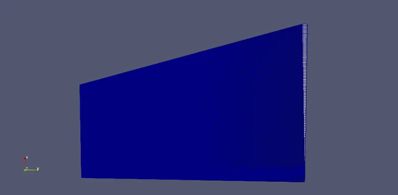
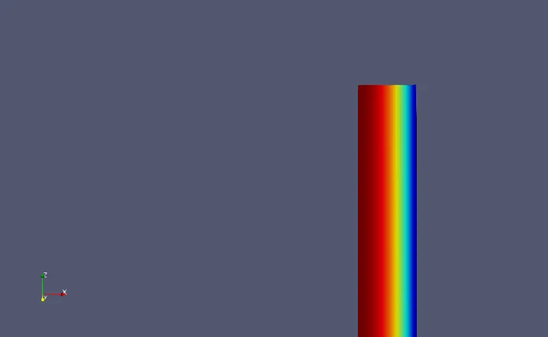
For a Wedge Angle = 2
Front View
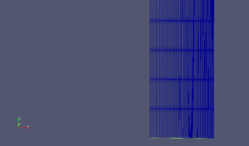
Sideview
Inlet
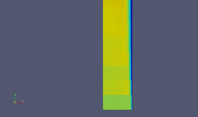
At Entry Length (2.52 m)
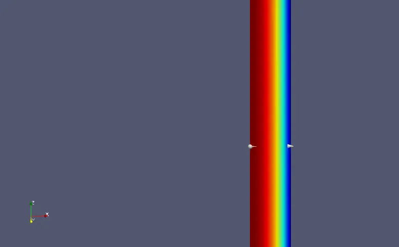
At outlet
Validating the Hydrodynamic Length with Numerical Results
According to the theory of Hydrodynamic length, the length is the distance from the inlet to the point within the pipe where the boundary layer grows from the wall to meet the axis of the pipe. In accordance with this, the shear stress would decrease from the inlet as the boundary layer grows and once the boundary layer grows and meets the axis of the pipe and the flow becomes fully developed, the shear stress would become constant.
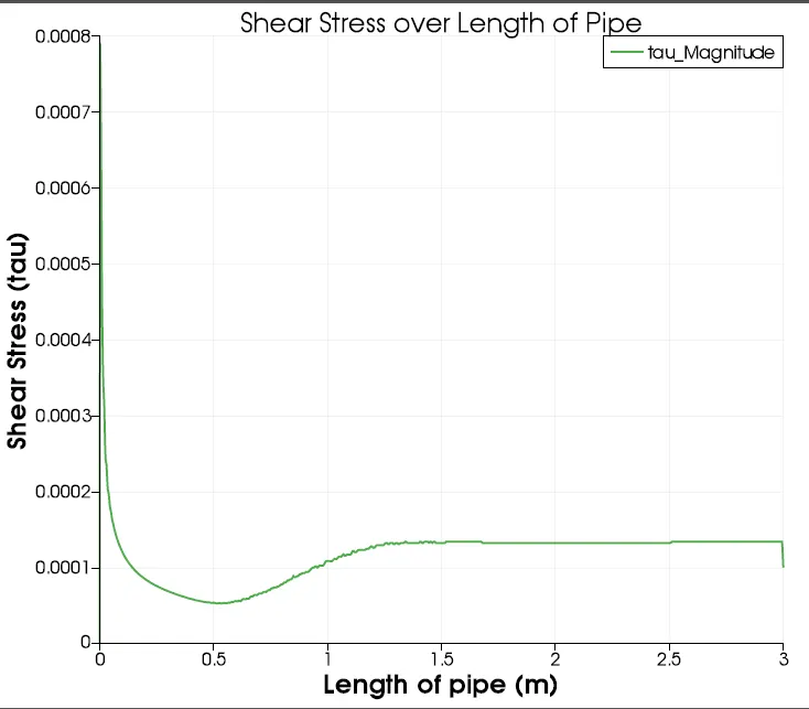
This plot of the shear stress calculated along the flow of the pipe shows that the shear stress becomes constant beyond approximately 2.52 m which would indicate that the flow has become fully developed beyond that point and therefore validated the entry length calculated by the empirical formula.
VELOCITY PROFILES:
Based on Numerical Results
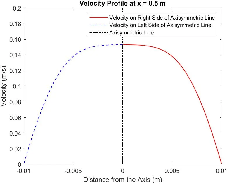
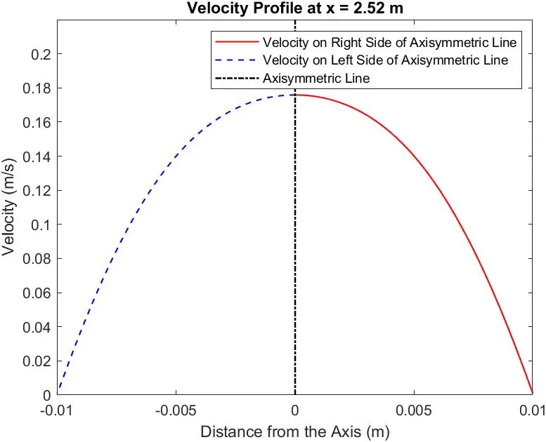
The following MATLAB code is used to plot the velocity profiles at both the inlet and at the entry length point (fully developed) using data extracted using the plot over line feature in ParaFOAM.
Code:
clear all
close all
clc

%To plot the velocity profile near the inlet
data = csvread('[email protected]',1,0);
mag_U = data(:,7);
arc_length = data(:,13);

%For the reflected section
ref_mag_U = mag_U;
ref_arc_length = -1.*arc_length;

origin = zeros(1,20);
y = linspace(0,0.20,20);

figure(1)
plot(arc_length,mag_U,'linewidth',1,'color','r');
hold on
plot(ref_arc_length,mag_U,'--','linewidth',1,'color','b');
plot(origin,y,'-.','linewidth',1.2,'color','k');
axis([-0.01 0.01 0 0.20])
legend('Velocity on Right Side of Axisymmetric Line','Velocity on Left Side of Axisymmetric Line');
xlabel('Distance from the Axis (m)');
ylabel('Velocity (m/s)');
title('Velocity Profile at x = 0.5 m');


%To plot the fully developed velocity profile

data2 = csvread('[email protected]',1,0);
mag_U = data2(:,7);
arc_length = data2(:,13);

%For the reflected section
ref_mag_U = mag_U;
ref_arc_length = -1.*arc_length;

origin = zeros(1,20);
y = linspace(0,0.20,20);

figure(2)
plot(arc_length,mag_U,'linewidth',1,'color','r');
hold on
plot(ref_arc_length,mag_U,'--','linewidth',1,'color','b');
plot(origin,y,'-.','linewidth',1.2,'color','k');
axis([-0.01 0.01 0 0.20])
legend('Velocity on Right Side of Axisymmetric Line','Velocity on Left Side of Axisymmetric Line');
xlabel('Distance from the Axis (m)');
ylabel('Velocity (m/s)');
title('Velocity Profile at x = 2.52 m');
PLOTS
Near the inlet
Fully developed (at entry length)
Based on Analytic Methods:
Based on the Hagen Poiseulle Formula
`v = R^2/(4mu)xx(dp)/(dx)xx[1 - (r/R)^2]`
`= v_(max)xx[1-(r/R)^2]`
Plotting the velocity profile based on this formula
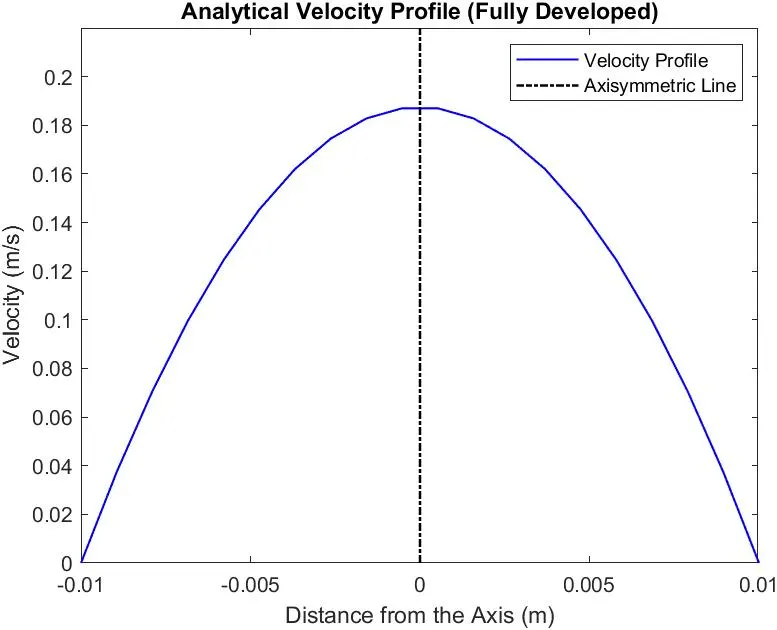
It is clear that there is a slight deviation between the maximum velocity derived analytically (0.1875 m/s) and the maximum velocity obtained numerically (0.1759 m/s)
Calculating the pressure drop
According to Hagen-Poiseulle
`trianglep = (32xxmuxxvxxL)/D^2`
`triangle p = 20.02` Pa
From the numerical solution
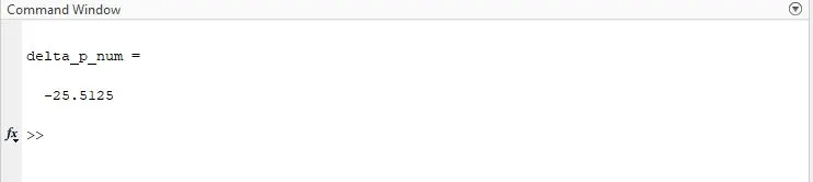
`trianglep = 25.51` Pa
Shear Stress
At the fully developed cross-section
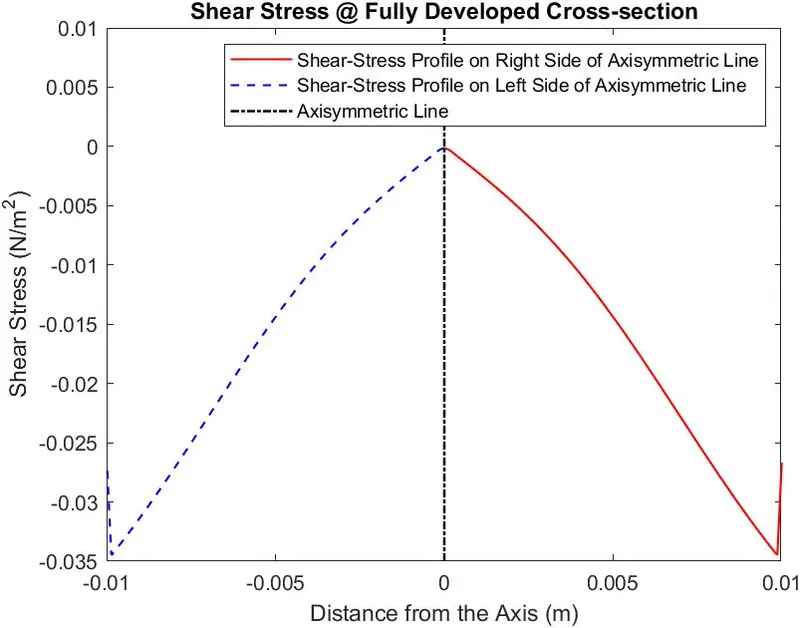
The shear stress at the cross-section shows that the shear stress is maximum at the walls due to the assumed no-slip condition and drops to 0 at the center of the pipe.