Simulation of a 1D Supersonic nozzle flow simulation using MacCormack Method

AIM:-

To use the MacCormack method to solve the 1-dimensional convergent-divergent nozzle flow problem with the initial conditions provided for both conservative and non-conservative forms of the governing equations.

THEORY:-

A convergent-divergent nozzle is a nozzle that has a decreasing (convergent) area till the throat (section of the minimum area) and then an increasing (divergent) area.

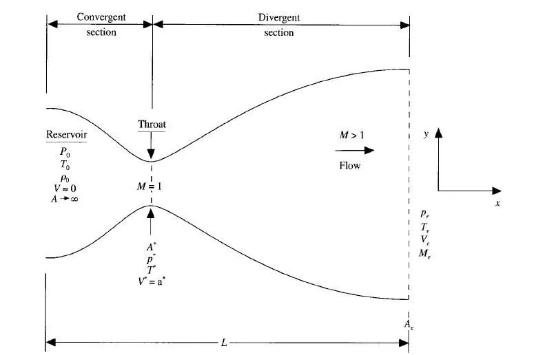
This is a 2D representation of a convergent-divergent nozzle. The flow enters the nozzle from a reservoir attached at the convergent end and it starts off as subsonic flow (speed of flow (v) < speed of sound (a)) and then reaches sonic flow at the throat and then becomes supersonic in the divergent section.

The Mach No. (M) is the ratio of the flow speed (v) to the speed of sound (a), so M<1 in the convergent section and M>1 in the divergent section.

The MacCormack method is an explicit finite difference method that is second-order accurate in both space and time that uses predictor and corrector to evaluate the solution.

In this problem, the conservative and non-conservative forms of the governing equations are solved using the MacCormack method. The governing equations consist of the continuity equation, momentum equations, and energy equations.

Non-Conservative Form

This is the form of the governing equations obtained when the control volume is assumed to be moving.

here, T represents temperature which is obtained by converting the specific energy (e) = C_v*T.

These are the non-dimensionalized form of the equations.

The initial conditions at time t=0 are given as,

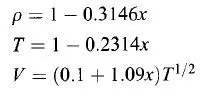
These equations represent the values of the density, temperature, velocity, and area at time t = 0 along the x-direction in the nozzle.

Conservative Form

This is the form of the governing equations obtained when the control volume is assumed to be stationary.

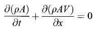
These are the non-dimensionalized form of the equations.

Then the equations are rearranged into a solutions vector U, the flux vector V, and the source term J. The elements of these new arrays are as follows:

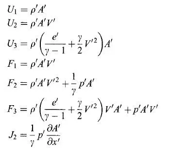
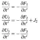
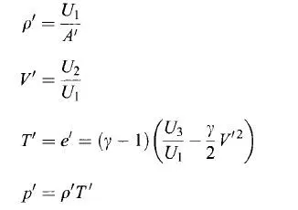
Here, the MacCormack method instead of solving for the primitive variables density (rho), temperature (T), and velocity (v) will solve for the new primary variables which are the elements of the solution vector (U), and once these are calculated the primitive variables can be derived from them as follows:

The system of equations for both conservative and non-conservative forms are hyperbolic in nature and so the CFL stability criterion that says that the Courant No. (C) should lie between 0 and 1. However, this criterion is for linear hyperbolic equations whereas the governing system of equations are non-linear hyperbolic equations so the criterion serves more as a guideline than a criterion. Using this principle, the time step (trianglet) should be calculated as such:

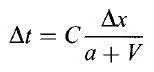
where a is the velocity of sound

v is the velocity of the flow.

METHOD:-

The main code

• The main code starts with defining the no. of elements in the domain and the no. of time steps to calculate for.
• The non-conservative form of the system of governing equations is solved first, starting with inputting the initial conditions of the system which are provided. The system is solved using a function called noncons, which takes in the no. of grid points, element size, initial conditions of the primitive variables, and the Courant no. (C_noncons) and gives the values of the primitive variables (rho, T, v, p) at each time step.
  
  
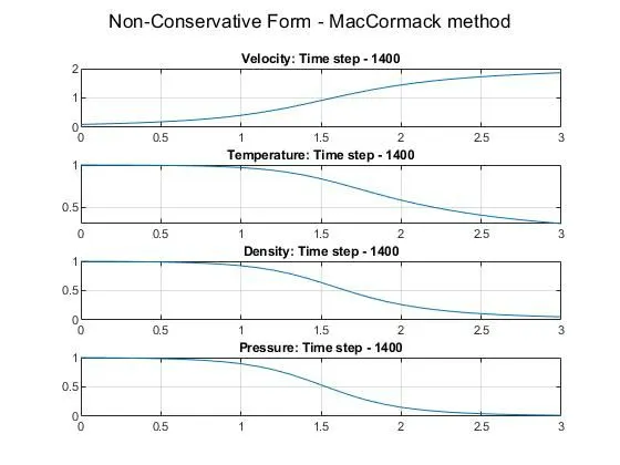
• This data is used to plot the values of the primitive variables at the steady-state condition which is achieved within the preset 1400 time steps. The data is also plotted within a for loop to see the time-wise variation of the primitive variables and this is used to create an animated video file.
  
  
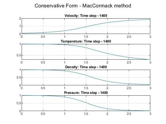
• The same process is carried out for the conservative form of the system of governing equations.
  
  
• The mass flow variation with time is compared between the conservative and non-conservative forms and the plots are used to create an animated video file.
  
  
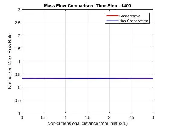
• Plots to compare the steady-state mass flow rates for each of the forms are also created.
  
  
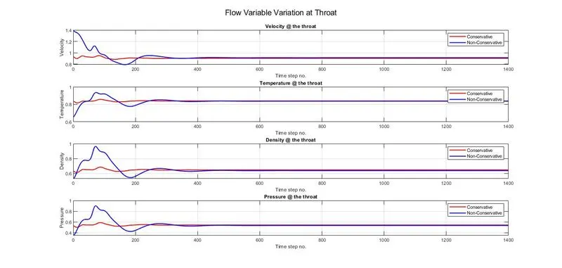
• Plots to compare the variation of primitive variables at the throat for both forms of the system of governing equations are also created.

%MacCormack method

clear all
close all
clc

%Inputs

n = 31; %No. of grid points
x = linspace(0,3,n);
dx = x(2) - x(1);
gamma = 1.4;


%Non-Conservative Form
%Initial Conditions (Non-dimensional)
rho = 1 - 0.3146*x;
T = 1 - 0.2314*x;
v = (0.1 + 1.09*x).*T.^(1/2);
A = 1 + 2.2.*(x - 1.5).^2;

x_throat = x(find(A == min(A(1,:))));

nt = 1400;
C_noncons = 0.5;
m = C_noncons.*(dx./((T.^0.5) + v));
dt = min(m(2:(n-1)));

%For Steady-state Plots

[rho_noncons,T_noncons,v_noncons,p_noncons,mflo_noncons,dt_noncons] = noncons(n,dx,gamma,rho,A,v,T,nt,C_noncons);
    

figure(1)
subplot(4,1,1)
sgtitle('Non-Conservative Form - MacCormack method')
%For velocity
plot(x,v_noncons(:,nt))
title(sprintf('Velocity: Time step - 1400'))
grid on
%For temperature
subplot(4,1,2)
plot(x,T_noncons(:,nt))
title(sprintf('Temperature: Time step - 1400'))
grid on
%For density
subplot(4,1,3)
plot(x,rho_noncons(:,nt))
title(sprintf('Density: Time step - 1400'))
grid on
%For pressure
subplot(4,1,4)
plot(x,p_noncons(:,nt))
title(sprintf('Pressure: Time step - 1400'))
grid on

%For Time-wise variation of the primitive variables
for k = 1:nt
    
   figure(2)
    subplot(4,1,1)
    sgtitle('Non-Conservative Form - MacCormack method')
    %For velocity
    plot(x,v_noncons(:,k))
    title(sprintf('Velocity: Time step - %d',k))
    grid on
    %For temperature
    subplot(4,1,2)
    plot(x,T_noncons(:,k))
    title(sprintf('Temperature: Time step - %d',k))
    grid on
    %For density
    subplot(4,1,3)
    plot(x,rho_noncons(:,k))
    title(sprintf('Density: Time step - %d',k))
    grid on
    %For pressure
    subplot(4,1,4)
    plot(x,p_noncons(:,k))
    title(sprintf('Pressure: Time step - %d',k))
    grid on
    
    N(k) = getframe(gcf);
    
end

% To create the animation videofile
movie(N)
filename = sprintf('Non-Conservative_Form.avi');
videofile = VideoWriter(filename,'Uncompressed AVI');
open(videofile)
writeVideo(videofile,N)
close(videofile)


%Conservative Form


%Initial Conditions (Non-dimensional)
for i = 1:n
    if x(i)<=0.5
    rho(i) = 1;
    T(i) = 1;
    elseif (0.5<x(i))&&(x(i)<=1.5)
        rho(i) = 1 - 0.366*(x(i) - 0.5);
        T(i) = 1 - 0.167*(x(i) - 0.5);
    elseif (1.5<x(i))&&(x(i)<= 3.5)
        rho(i) = 0.634 - 0.3879*(x(i) - 1.5);
        T(i) = 0.833 - 0.3507*(x(i) - 1.5);
    end
end

A = 1 + 2.2.*(x - 1.5).^2;
v = 0.59./(rho.*A); %Assuming that mass flow is constant initially


nt = 1400;
C_cons = 0.5;
m = C_cons.*(dx./((T.^0.5) + v));
dt = min(m(2:(n-1)));

%For Steady-state Plots
[rho_cons,T_cons,v_cons,p_cons,mflo_cons,dt_cons] = cons(n,dx,gamma,rho,A,v,T,nt,C_cons);


%Steady-state Plots
figure(3)
subplot(4,1,1)
sgtitle('Conservative Form - MacCormack method')
%For velocity
plot(x,v_cons(:,nt))
title(sprintf('Velocity: Time step - 1400'))
grid on
%For temperature
subplot(4,1,2)
plot(x,T_cons(:,nt))
title(sprintf('Temperature: Time step - 1400'))
grid on
%For density
subplot(4,1,3)
plot(x,rho_cons(:,nt))
title(sprintf('Density: Time step - 1400'))
grid on
%For pressure
subplot(4,1,4)
plot(x,p_cons(:,nt))
title(sprintf('Pressure: Time step - 1400'))
grid on




%For the Time-wise variation of the primary variables

for k = 1:nt
       figure(2)
    subplot(4,1,1)
    sgtitle('Conservative Form - MacCormack method')
    %For velocity
    plot(x,v_cons(:,k))
    title(sprintf('Velocity: Time step - %d',k))
    grid on
    %For temperature
    subplot(4,1,2)
    plot(x,T_cons(:,k))
    title(sprintf('Temperature: Time step - %d',k))
    grid on
    %For density
    subplot(4,1,3)
    plot(x,rho_cons(:,k))
    title(sprintf('Density: Time step - %d',k))
    grid on
    %For pressure
    subplot(4,1,4)
    plot(x,p_cons(:,k))
    title(sprintf('Pressure: Time step - %d',k))
    grid on
    
    K(k) = getframe(gcf);
end

% To create the animation videofile
movie(K)
filename = sprintf('Conservative_Form.avi');
videofile = VideoWriter(filename,'Uncompressed AVI');
open(videofile)
writeVideo(videofile,K)
close(videofile)




%Comparing the mass flow rates at different time steps

for k = 1:nt
    figure(5)
    clf;
    plot(x,mflo_cons(:,k),'r','linewidth',1.5)
    hold on
    plot(x,mflo_noncons(:,k),'b','linewidth',1.5)
    grid on
    axis([0 3 -1 3]);
    
    legend('Conservative','Non-Conservative')
    title(sprintf('Mass Flow Comparison: Time Step - %d',k))
    xlabel('Non-dimensional distance from inlet (x/L)')
    ylabel('Mass Flow Rate')
    
    M(k) = getframe(gcf);
    
end


% To create the animation videofile
movie(M)
filename = sprintf('Mass_Flow_Comp.avi');
videofile = VideoWriter(filename,'Uncompressed AVI');
open(videofile)
writeVideo(videofile,M)
close(videofile)

%Comparing the normalized flow rates at steady state

mflo_throat_cons = mflo_cons(find(x == x_throat),nt);
mflo_throat_noncons = mflo_noncons(find(x == x_throat),nt);

norm_mflo_cons_ss = mflo_cons(:,nt).*mflo_throat_cons;
norm_mflo_noncons_ss = mflo_noncons(:,nt).*mflo_throat_noncons;

figure(6)
plot(x,norm_mflo_cons_ss,'r','linewidth',2)
hold on
plot(x,norm_mflo_noncons_ss,'b','linewidth',1.5)
grid on
axis([0 3 -1 3]);
legend('Conservative','Non-Conservative')
title(sprintf('Mass Flow Comparison: Time Step - 1400'))
xlabel('Non-dimensional distance from inlet (x/L)')
ylabel('Normalized Mass Flow Rate')

%For variation of flow variables at different time steps at the throat

t = [1:1:1400];

figure(7)
subplot(4,1,1)
sgtitle('Flow Variable Variation at Throat')
%For velocity
plot(t,v_cons(find(x == x_throat),:),'r','linewidth',1.5)
hold on 
plot(t,v_noncons(find(x == x_throat),:),'b','linewidth',1.5)
title(sprintf('Velocity @ the throat'))
grid on
legend('Conservative','Non-Conservative')
xlabel('Time step no.')
ylabel('Velocity')
%For temperature
subplot(4,1,2)
plot(t,T_cons(find(x == x_throat),:),'r','linewidth',1.5)
hold on 
plot(t,T_noncons(find(x == x_throat),:),'b','linewidth',1.5)
title(sprintf('Temperature @ the throat'))
grid on
legend('Conservative','Non-Conservative')
xlabel('Time step no.')
ylabel('Temperature')
%For density
subplot(4,1,3)
plot(t,rho_cons(find(x == x_throat),:),'r','linewidth',1.5)
hold on 
plot(t,rho_noncons(find(x == x_throat),:),'b','linewidth',1.5)
title(sprintf('Density @ the throat'))
grid on
legend('Conservative','Non-Conservative')
xlabel('Time step no.')
ylabel('Density')
%For pressure
subplot(4,1,4)
plot(t,p_cons(find(x == x_throat),:),'r','linewidth',1.5)
hold on 
plot(t,p_noncons(find(x == x_throat),:),'b','linewidth',1.5)
title(sprintf('Pressure @ the throat'))
grid on
legend('Conservative','Non-Conservative')
xlabel('Time step no.')
ylabel('Pressure')

For the non-conservative form function (noncons)

• The function takes the inputs of the no. of grid points, element size, initial conditions of the primitive variables, and the Courant no. (C_noncons) and gives the values of the primitive variables (rho, T, v, p), and mass flow at each time step.

function [rho_noncons,T_noncons,v_noncons,p_noncons,mflo_noncons,dt_noncons] = noncons(n,dx,gamma,rho,A,v,T,nt,C_noncons)

%MacCormack method
%Non-Conservative Form


m = C_noncons.*(dx./((T.^0.5) + v));
dt = min(m(2:(n-1)));




for k = 1:nt
    
    rho_initial = rho;
    v_initial = v;
    T_initial = T;
    
    %Predictor
    for i = 2:n-1
    
    dv_dx = (v(i+1) - v(i))/dx;
    dlogA_dx = (log(A(i+1))-log(A(i)))/dx;
    drho_dx = (rho(i+1)-rho(i))/dx;
    dT_dx = (T(i+1)-T(i))/dx;
    
    %Continuity equation
    
    drho_dt_p(i) = -rho(i)*dv_dx - rho(i)*v(i)*dlogA_dx - v(i)*drho_dx;
    
    %Momentum equation
    
    dv_dt_p(i) = -v(i)*dv_dx - (1/gamma)*(dT_dx + (T(i)/rho(i))*(drho_dx));
    
    %Energy equation
    
    dT_dt_p(i) = -v(i)*dT_dx - (gamma - 1)*T(i)*(dv_dx + v(i)*dlogA_dx);
    
    %Solution Update
    
    rho(i) = rho(i) + drho_dt_p(i)*dt;
    v(i) = v(i) + dv_dt_p(i)*dt;
    T(i) = T(i) + dT_dt_p(i)*dt;
    
    end
    
    
    %Corrector
    for i = 2:n-1
    
    dv_dx = (v(i) - v(i-1))/dx;
    dlogA_dx = (log(A(i))-log(A(i-1)))/dx;
    drho_dx = (rho(i)-rho(i-1))/dx;
    dT_dx = (T(i)-T(i-1))/dx;
    
    %Continuity equation
    
    drho_dt_c(i) = -rho(i)*dv_dx - rho(i)*v(i)*dlogA_dx - v(i)*drho_dx;
    
    %Momentum equation
    
    dv_dt_c(i) = -v(i)*dv_dx - (1/gamma)*(dT_dx + (T(i)/rho(i))*(drho_dx));
    
    %Energy equation
    
    dT_dt_c(i) = -v(i)*dT_dx - (gamma - 1)*T(i)*(dv_dx + v(i)*dlogA_dx);
    
    
    end
    
    %Getting the time averaged derivative
    
    drho_dt = 0.5*(drho_dt_p + drho_dt_c);
    dv_dt = 0.5*(dv_dt_p + dv_dt_c);
    dT_dt = 0.5*(dT_dt_p + dT_dt_c);
    
    %Final solution update
    
    for i = 2:n-1
        
        rho(i) = rho_initial(i) + drho_dt(i)*dt;
        v(i) = v_initial(i) + dv_dt(i)*dt;
        T(i) = T_initial(i) + dT_dt(i)*dt;
        
    end
    
    %Applying boundary conditions
    
    %Inlet
    v(1) = 2*v(2) - v(3);
    
    %Outlet
    v(n) = 2*v(n-1) - v(n-2);
    rho(n) = 2*rho(n-1) - rho(n-2);
    T(n) = 2*T(n-1) - T(n-2);
    
    %Mass Flow Rate
    mflo(:,k) = rho.*v.*A;
    %Pressure
    p_noncons(:,k) = rho.*T;
    
    v_noncons(:,k) = v;
    rho_noncons(:,k) = rho;
    T_noncons(:,k) = T;
    
    
end



mflo_noncons = mflo;
dt_noncons = dt;

end

For the conservative form function (cons)

• The function takes the inputs of the no. of grid points, element size, initial conditions of the primitive variables, and the Courant no. (C_cons) and gives the values of the primitive variables (rho, T, v, p), and mass flow at each time step.

function [rho_cons,T_cons,v_cons,p_cons,mflo_cons,dt_cons] = cons(n,dx,gamma,rho,A,v,T,nt,C_cons)

%Consevative Form

%MacCormack method

m = C_cons.*(dx./((T.^0.5) + v));
dt = min(m(2:(n-1)));

%Defining the solution vector

u1 = rho.*A;
u2 = rho.*A.*v;
u3 = rho.*A.*((T/(gamma - 1))+((gamma/2)*v.^2));

for k = 1:nt
    
    u1_initial = u1;
    u2_initial = u2;
    u3_initial = u3;
    
    
    
    %Flux vector terms in terms of u1, u2 and u3
    f1 = u2;
    f2 = ((u2.^2)./u1) + ((gamma - 1)/gamma)*(u3 - (gamma/2)*((u2.^2)./u1));
    f3 = gamma*((u2.*u3)./u1) - ((gamma*(gamma - 1))/2)*((u2.^3)./(u1.^2));

    %Predictor step
    for i = 2:n-1

        dA_dx = (A(i+1)-A(i))/dx;

        j2 = (1/gamma)*rho(i)*T(i)*dA_dx;


        %Continuity equation
        du1_dt_p(i) = -(f1(i+1) - f1(i))/dx;

        %Momentum equation
        du2_dt_p(i) = j2 - (f2(i+1) - f2(i))/dx;

        %Energy equation
        du3_dt_p(i) = -(f3(i+1) - f3(i))/dx;


        %Solution update 

        u1(i) = u1(i) + du1_dt_p(i)*dt;
        u2(i) = u2(i) + du2_dt_p(i)*dt;
        u3(i) = u3(i) + du3_dt_p(i)*dt;

    end 

    %Predicted values of primitive variables

    rho_p = u1./A;
    v_p = u2./u1;
    T_p = (gamma - 1)*((u3./u1) - ((gamma/2)*(v_p.^2)));


    f1 = u2;
    f2 = ((u2.^2)./u1) + ((gamma - 1)/gamma)*(u3 - (gamma/2)*((u2.^2)./u1));
    f3 = gamma*((u2.*u3)./u1) - ((gamma*(gamma - 1))/2)*((u2.^3)./(u1.^2));

    %Corrector step

    for i = 2:n-1


        dA_dx = (A(i)-A(i-1))/dx;

        j2 = (1/gamma)*rho_p(i)*T_p(i)*dA_dx;


        %Continuity equation
        du1_dt_c(i) = -(f1(i) - f1(i-1))/dx;

        %Momentum equation
        du2_dt_c(i) = j2 - (f2(i) - f2(i-1))/dx;

        %Energy equation
        du3_dt_c(i) = -(f3(i) - f3(i-1))/dx;

    end


    %Getting time averaged derivative

    du1_dt = 0.5*(du1_dt_p + du1_dt_c);
    du2_dt = 0.5*(du2_dt_p + du2_dt_c);
    du3_dt = 0.5*(du3_dt_p + du3_dt_c);

    %Final solution

    for i = 2:n-1
        u1(i) = u1_initial(i) + du1_dt(i)*dt;
        u2(i) = u2_initial(i) + du2_dt(i)*dt;
        u3(i) = u3_initial(i) + du3_dt(i)*dt;
    end

    %Boundary Conditions
    %Inlet
    u1(1) = rho_p(1)*A(1);
    u2(1) = 2*u2(2) - u2(3);
    v_p(1) = u2(1)/u1(1);
    u3(1) = u1(1)*((T_p(1)/(gamma-1)) + (gamma/2)*v_p(1)^2);  

    %Outlet
    u1(n) = 2*u1(n-1) - u1(n-2);
    u2(n) = 2*u2(n-1) - u2(n-2);
    u3(n) = 2*u3(n-1) - u3(n-2);
    
    rho = u1./A;
    v = u2./u1;
    T = (gamma - 1)*((u3./u1) - (gamma/2)*(v.^2));
    p = rho.*T;
    mflo(:,k) = rho.*A.*v;
    
    rho_cons(:,k) = rho;
    v_cons(:,k) = v;
    T_cons(:,k) = T;
    p_cons(:,k) = p;
    
    

end

mflo_cons = mflo;
dt_cons = dt;

end

PLOTS:-

Steady-state distribution of primitive variables for

Non-Conservative Form of equations

Conservative Form of equations

Time-wise variation of primitive variables

For Non-Conservative Form of equations

Click here

For Conservative Form of equations

Click here

For time wise variation of primitive variables at the throat

Variation of mass flow rate distribution at different time steps

For both Non-Conservative & Conservative Form of equations

Click here

Comparison of Normalized mass flow rate distributions of both forms at steady state

Grid Independence Study

To study the effect of the grid on the solution we need to change the size of the grid and see if it alters the solution significantly

The values at the throat node at the last time step are compared

	Density	Temperature	Pressure	Mach No.
Exact Solution	0.634	0.833	0.528	1
Conservative Solution (n = 31)	0.6485	0.839	0.5441	0.9025
Non-Conservative Solution(n = 31)	0.6387	0.8365	0.5342	0.914
Non-Conservative Solution (n = 61)	0.6377	0.8354	0.5327	0.9138

It is seen that even when the no. of grid points are increased there is no significant change in the solution obtained. Hence the solution is grid-independent.