FVM Literature Review

Finite Volume Method (FVM) is a discretization method used to convert integral forms of governing equations into algebraic equations. This method is inherently conservative due to the use of the integral forms of the equations.

The properties of the discretization method required for the numerical results of the computation to be physically realistic are:

• Conservativeness - the flux of a property (`phi`) leaving a face should be equal to the flux of `phi`entering the adjacent face.
  
  
• Boundedness - the values of the property `phi` during discretization is calculated at the cell centers/centroids and the value at this internal node should be in between (bounded by) the upper and lower limits of the values of the property `phi` given at the boundaries.
  
  
• Transportiveness - this means that the values obtained at the nodes should make sense from a advection-diffusion standpoint, i.e., if the problem is advection dominant (where there is bulk fluid motion) the values should be reflective of the direction of flow as in the value of `phi` at a node will be mainly affected by the node upstream of it due to the flow direction, whereas if the problem is diffusion dominant then the values at each node will be equally affected by the values at adjacent nodes.
  The Peclet Number (Pe) is the ratio of advection flux to diffusive flux and is used to represent the dominance of one over the other.

Differences between FDM and FVM

• In FDM, the differential form of the governing equations are used whereas in FVM the integral form of the governing equations are used.
  
  
• In FDM, the governing equations are valid at infinitesimal control volumes called grid points/nodes which the domain is divided into, and the unit consisting of 2 grid points and the region of the domain in between them is called an element.
  In FVM, the governing equations are valid across finite-sized control volumes called cells and the values of the field variables are calculated at the centroid of the cell.
• FDM is difficult to apply to complex geometries because it is difficult to make sure that the boundaries lie on the grid points whereas FVM is more suitable for complex geometries since they can easily ensure that the cell center lies on the boundaries of the complex geometries. The boundaries are important because they contain the known conditions and are essential for arriving at the algebraic forms of the governing equations.
  
  

Interpolation Schemes

These are the methods used to find the values of field variables at points other than the cell centers (here, w, and e) such as at the faces of the control volume (Cell) which are required to discretize the advection-diffusion equation using FVM. The advection-diffusion equation is derived from the general transport equation that does not have a source and is in steady-state condition.

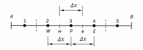
The interpolation methods are:

• Linear Interpolation/Central Differencing
• Upwind Differencing
• Second-Order Upwind Differencing/Linear Upwind Differencing (LUD)/Beam-Warming
• Hybrid
• TVD

Note: Throughout the explanation, the property `phi` is considered to be temperature represented by T.

Linear Interpolation/Central Differencing

This method is used for situations that are diffusion dominant (without convection, like in conduction problems) and the value is influenced equally by adjacent points.

`T_e = (T_E*trianglex_(Pe) + T_P*trianglex_(eE))/(trianglex_(eE)+trianglex_(Pe))` for non-uniform grid`

if the grid is uniform (as shown)

`T_e = (T_P+T_E)/2`

Advantages

• Has second-order accuracy
• It satisfies the boundedness property for Pe<2
• Conservativeness satisfied

Disadvantages

• The Transportiveness property is not satisfied since the scheme doesn't recognize flow direction.
• Only gives accurate results for Pe<2. Unstable.

Upwind Differencing

This method is used for situations that are advection dominant (like in convection heat transfer problems) where there is a bulk movement of fluid in a particular direction. The value at the required intermediate point is only affected by the cell center value upwind of the intermediate point with respect to the direction of fluid movement.

`T_e={T_P if u>0; T_E if u<0`

Advantages

• Conservativeness satisfied
• Unconditionally satisfies boundedness condition
• It satisfies the transportiveness property

Disadvantages

• First-order accurate
• produces errors if the flow is not aligned along the grid lines (false diffusion)
• Creates oscillations

Hybrid

This is a combination of Central Differencing (CD) and First Order Upwind (FOU) Differencing which are chosen between based on the Peclet number (Pe).

If `Pe<2`then CD is used

`Pe>=2`then FOU is used

This method combines the benefits of both CD and FOU schemes.

Linear Upwind Differencing (LUD)/Second Order Upwinding (SOU)

This is a second-order accurate version of the upwind differencing method which is first-order accurate. This is also applicable in convection dominant flows.

if u>0

`T_e = T_P + (T_P-T_W)/2`

if u<0

`T_e = T_E + (T_E-T_(E E))/2`

Advantages

• It is second-order accurate.
• Unconditionally satisfies boundedness condition
• It satisfies the transportiveness property

Disadvantages

• In highly convective flows (High Pe) the scheme is oscillatory (unbounded)

QUICK (Quadratic Upwind Interpolation for Convective Kinematics)

In this method, the values of 3 adjacent computational nodes (2 upstream W and WW and 1 downstream E) are taken and quadratically interpolated to get the value at the intermediate points.

`T_e = 6/8*T_P+3/8*T_E-1/8*T_W`

`T_w = 3/8*T_P+6/8*T_W-1/8*T_(WW)`

Advantages

• It is third-order accurate.
• Conservative
• Unconditionally satisfies boundedness condition
• It satisfies the transportiveness property since 2 upstream and 1 downstream

Disadvantages

• For high Pe, there are stability problems leading to unbounded solutions this leads to overshoots and undershoots.
• Conditionally stable

Total Variation Diminishing (TVD) Schemes

TVD schemes are schemes that do not create overshoots or undershoots, unlike the QUICK and higher-order methods. It leads to stable, non-oscillatory, and bounded schemes. The tendency to oscillate is counteracted by the limiter functions (`psi`). These functions detect strong gradients or changes in slope and switches locally to lower resolution (first-order accuracy, upwind), and everywhere else they will retain the higher resolution.

`T_e = T_P+1/2*psi(r).(T_E-T_P)`

Here the limiting function (`psi`) is represented as a function of r which is the ratio of upwind side gradient to the downwind side gradient of the property which here is T, i.e,

`r = (T_P - T_W)/(T_E-T_P)`

Based on this definition it can be seen that the limiting function for

For Upwind Differencing/FOU,

`psi(r) = 0`

For Central Differencing

`psi(r) = 1`

For Linear Upwind Differencing (LUD)

`psi(r) = r`

For QUICK,

`psi(r) = (3+r)/4`