Genetic Algorithm
AIM:-
To identify the maximum value of the stalagmite function using the inbuilt MATLAB genetic algorithm function while also studying the behavior of the genetic algorithm during 3 different cases:
- Unbounded search-space.
- Bounded search-space.
- Increased generated population space.
INTRODUCTION:-
Stalagmite function
The stalagmite function is a function that when plotted resembles stalagmites, which are spires of rock that grow from the ground upwards usually found in caves. The stalagmite function (F(x))is as follows
`F(x) = f_(1,x)*f_(2,x)*f_(1,y)*f_(2,y)`
where
`f_(1,x) = (sin(5.1*pi*x+0.5))^6`
`f_(1,y) = (sin(5.1*pi*y+0.5))^6`
`f_(2,x)=exp((-4*log(2)*(x-0.0667)^2)/(0.64))`
`f_(2,y)=exp((-4*log(2)*(y-0.0667)^2)/(0.64))`
Genetic Algorithm
The genetic algorithm is an optimization technique that is named and works based on Darwin's theory of a natural selection based evolution. They use concepts from evolutionary biology to search for global minimums. They work as follows:
- First, the algorithm generates a random population of the variables in the function to be optimized and evaluate the value of the function at these points. The fitness of the members within this population are evaluated using a fitness function (which checks how close the output of each member is to the optimal/minimum output). The members of the population that provide smaller output will have a higher fitness value since the objective is to find the minimum value.
- The members with better fitness values are selected as parents (using a variety of methods such as the Cost Roulette Wheel, Stochastic Universal Sampling, Rank Roulette Wheel, Tournament Selection, etc.) and these parents are used to create the next generation of the population through methods such as selection, crossover, and mutation.
- Selection is when parents are selected to be retained from one generation to the next because of their high fitness.
- Crossover is when the similarities in the characters of the selected parents from one generation are combined to create members of the population in the next generation.
- Mutation is when random variables in the parents are changed (mutated) and used to create members of the subsequent generation. This helps spread the population better and avoid falling into local minima.
- This process is carried out for several generations until the optimum fitness value gets repeated and then it is assumed to be the optimum member.
METHODOLOGY:-
For the stalagmite function:-
The stalagmite function is created within a separate MATLAB function named stalagmite.m and is accessed from within the main program as required.
The code just carries out the function as described above.
It takes in an input vector and outputs the value of the stalagmite function at that point. However since the genetic algorithm obtains the minimum value of a function and we require the maximum value, the stalagmite function here is defined as the negative of the actual stalagmite function.
For the genetic algorithm portion:-
The code just creates the input vector within the defined space of x and y and then runs and plots the genetic algorithm for each of the 3 cases mentioned above. The time taken for each case is also measured using the tic-toc commands.
STEPS:-
For the genetic algorithm portion:-
- The code starts with defining the space within which the stalagmite function exists. The set of x and y values between the range of 0 and 0.6 is obtained using the linspace command.
x = linspace(0,0.6,150);
y = linspace(0,0.6,150); - The number of iterations to be carried out is also defined as num_cases.
- The points on the x-y plane are plotted using the meshgrid function.
[xx yy] = meshgrid(x,y); - Then the input values are created and the stalagmite function (f) is used to calculate the value of f at each of these points using 2 for loops running between 1 and the number of x/y elements by using the stalagmite function.
for i = 1:length(xx)
for j = 1:length(yy)
input_vector(1) = xx(i,j);
input_vector(2) = yy(i,j);
f(i,j) = stalagmite(input_vector);
end
end
The values of f obtained are stored in the f matrix. - For case 1 - Unbounded search-space
The genetic algorithm is run using a for loop that iterates it for chosen number of times (num_cases) and the values of the optimal f value and its corresponding position are stored within the fval, x_opt and y_opt vectors respectively.
tic
for i = 1:num_cases
%Genetic algorithm code
[inputs, fval(i)] = ga(@stalagmite,2);
%Storing the positions of the optimum values in each iteration
x_opt(i) = inputs(1);
y_opt(i) = inputs(2);
end
study1_time = toc
Then the stalagmite function is plotted along with the optimum points obtained and also, the optimum f value (fval) is plotted for each iteration.
The tic-toc commands are used on either side of the for loop to calculate the amount taken for the defined number of iterations and this is stored in study1_time. - For case 2 - Bounded search-space
Same as above but here in order to bound the search space, the upper and lower bounds of the x and y values are inputted into the genetic algorithm command as follows.
[inputs, fval(i)] = ga(@stalagmite,2,[],[],[],[],[0;0],[1;1]);
here, the lower bound is given as 0 for both x & y and the upper bound is given as 1 for both x & y.
Then the time taken is calculated and the same plots are made as in the previous case. - For case 3 - Increased generated population space.
Here, in addition to the upper and lower bounds, the generated population size is increased.
This is done using the optimoptions command
options = optimoptions('ga');
options = optimoptions(options,'PopulationSize',300);
This defined the generated population size as 300 members.
And the genetic algorithm command varies as follows
[input,fval(i)] = ga(@stalagmite,2,[],[],[],[],[0;0],[1;1],[],[],options);
The rest of the code remains the same as in case 1.
CODE:-
For the stalagmite function:-
function [f]=stalagmite(input_vector)

x=input_vector(1);
y=input_vector(2);

f1=(sin(5.1*pi*x+0.5))^6;
f2=(sin(5.1*pi*y+0.5))^6;
f3=exp((-4*log(2)*(x-0.0667)^2)/(0.64));
f4=exp((-4*log(2)*(y-0.0667)^2)/(0.64));

f= -(f1*f2*f3*f4);
end
For the genetic algorithm portion:-
close all
clear all
clc

x = linspace(0,0.6,150);
y = linspace(0,0.6,150);
num_cases = 50;

input_vector = [0 0];

%Creating a 2D mesh
[xx yy] = meshgrid(x,y);


%Create the input vector
for i = 1:length(xx)
    for j = 1:length(yy)
        input_vector(1) = xx(i,j);
        input_vector(2) = yy(i,j);
        f(i,j) = stalagmite(input_vector);
    end
end

tic
%Study - 1 Statistical Behaviour
for i = 1:num_cases
    %Genetic algorithm code
    [inputs, fval(i)] = ga(@stalagmite,2);
    %Storing the positions of the optimum values in each iteration
    x_opt(i) = inputs(1);
    y_opt(i)  = inputs(2);
end

study1_time = toc

figure(2)
%3D plot with f value along z axis
subplot(2,1,1)
hold on
surf (xx,yy,-f)
xlabel('x value')
ylabel('y value')
shading interp

plot3(x_opt,y_opt,-fval,'marker','o','markersize',5,'markerfacecolor','r')
title ('Unbounded Inputs')

subplot(2,1,2)
plot(-fval)
xlabel('Iterations')
ylabel('Function Maximum')

tic
%Study - 2 Statistical study with upper and lower bounds

for i = 1:num_cases
    [inputs, fval(i)] = ga(@stalagmite,2,[],[],[],[],[0;0],[1;1]);
    %Storing the positions of the optimum values in each iteration
    x_opt(i) = inputs(1);
    y_opt(i)  = inputs(2);
end
study2_time = toc

figure(1)
%3D plot with f value along z axis
subplot(2,1,1)
hold on
surf (xx,yy,-f)
xlabel('x value')
ylabel('y value')
shading interp

plot3(x_opt,y_opt,-fval,'marker','o','markersize',5,'markerfacecolor','r')
title ('Bounded Inputs')

subplot(2,1,2)
plot(-fval)
xlabel('Iterations')
ylabel('Function Maximum')


% Study - 3 Increasing the population size in each generation
options = optimoptions('ga');
options = optimoptions(options,'PopulationSize',300);

tic
for i = 1:num_cases
    [input,fval(i)] = ga(@stalagmite,2,[],[],[],[],[0;0],[1;1],[],[],options);
    x_opt(i) = input(1);
    y_opt(i) = input(2);
end
study3_time = toc

figure(3)
%3D plot with f value along z axis
subplot(2,1,1)
hold on
surf (xx,yy,-f)
xlabel('x value')
ylabel('y value')
shading interp

plot3(x_opt,y_opt,-fval,'marker','o','markersize',5,'markerfacecolor','r')
title ('Bounded Inputs')

subplot(2,1,2)
plot(-fval)
xlabel('Iterations')
ylabel('Function Maximum')
OUTPUT:-
CASE 1 - UNBOUNDED SEARCH-SPACE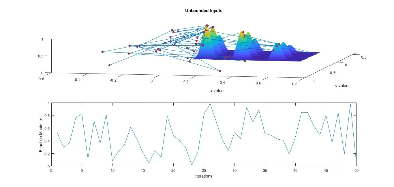
These are the output plots for case 1.
Points to note:
- There are a large number of points in the 3D plot that vary widely and some exist outside of the pre-defined limits of x and y where the stalagmite function is plotted. This is because these points are randomly generated.
- The function minimum varies a lot in each iteration and doesn't give a clear picture as to which value is actually the global minimum.
- The time taken for study 1 is 4.5 seconds.
CASE 2 - BOUNDED SEARCH-SPACE
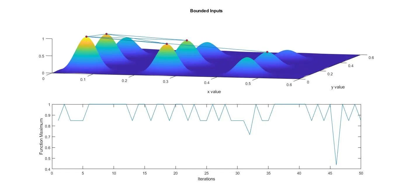
These are the output plots for case 2.
Points to note:
- Here the plotted points (in red) are not as widely distributed in the x-y plane and they exist only within the lower and upper bound that was defined as 0 and 1 for both x and y. This has helped the genetic algorithm spot the minima values within the search space better.
- The function minimum here also varies quite a bit but it oscillates between 0.85 and 1, with drops to 0.7 and 0.45.
- The time taken for study 2 is 5.22 seconds.
CASE 3 - INCREASED GENERATED POPULATION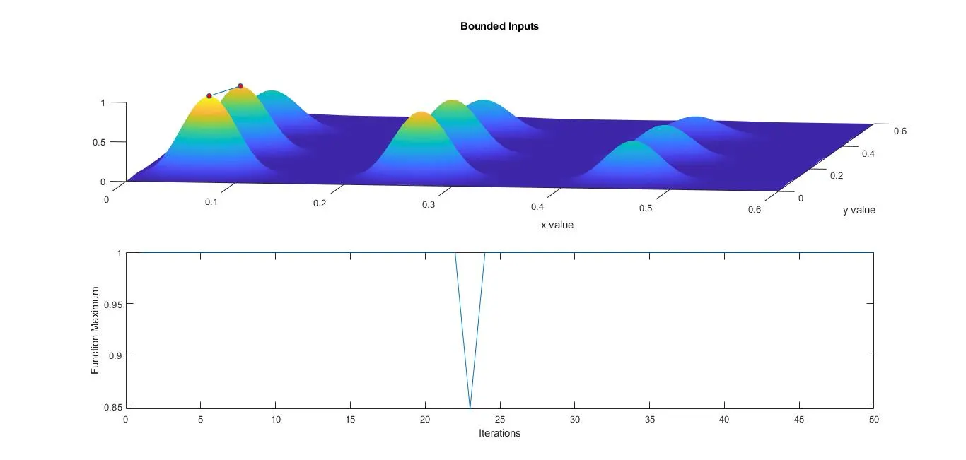
These are the output plots for case 3.
Points to note:
- Here the distribution of the optimum points of each iteration is more focussed and close to the global minima this is due to the increased population size in each generation allowing a wider range of points to be evaluated in each generation and therefore making the genetic algorithm get closer to the true global minima in each iteration.
- The function minimum here stays mostly at 1 except for a drop to 0.85 once in the 50 iterations.
- The time taken for study 3 is 19.5 seconds.
Hence, the maximum value can be assumed to be 1, which is found at x = y = 0.0668.