Week 5 - Curve fitting

1. popt – gives the optimal coefficients of the function to be fitted to the data points. pcov – it’s a square matrix whose diagonal elements gives an idea about the dependence of the coefficients for the fitted function. Larger the values means the variation of the coefficients are larger, meaning even if the coefficients are changed or adjusted the fitted function will not change much.

2. array(temperature) sends the values of the variable temperature in array format.

3. * in *popt mentions the program to take all the values present in the popt variable.

4. Main program for curve fitting using linear and cubic function. Working of the code has been explained with comments

import matplotlib.pyplot as plt
import math
import numpy as np
import statistics
from scipy.optimize import curve_fit

#curve fit function
def lin_func(t, a, b):
	return a*pow(t,1)+ b

def cubic_func(t, l, m, n, o):
	return l*pow(t,3) + m*pow(t,2) + n*t + o


#reading therm data file
def read_file():
	temperature = []
	cp = []
	for line in open('data', 'r'):
		values = line.split(',')
		temperature.append(float(values[0]))
		cp.append(float(values[1]))
	return [temperature, cp]



#main program
temperature, cp = read_file() #reading temperature and cp from data file
popt_lin, pcov_lin = curve_fit(lin_func, temperature, cp) #optimum coefficients for linear func
popt_cubic, pcov_cubic = curve_fit(cubic_func, temperature, cp) #optimum coefficients for cubic func
fit_cp_lin =  lin_func(np.array(temperature), *popt_lin) #linear fitted cp values
fit_cp_cubic =  cubic_func(np.array(temperature), *popt_cubic) # cubic fitted cp values



#calculation of fit of the curve for linear function
y1 = []
y2 = []
for i in range(0,len(fit_cp_lin)):
	y1.append(pow((fit_cp_lin[i]-cp[i]),2))
	y2.append(pow((fit_cp_lin[i]-statistics.mean(cp)),2))

SSE_lin = sum(y1) #sum of square errors
SSR_lin = sum(y2) #sum of square regression
r_square_lin = SSR_lin/(SSR_lin+SSE_lin) #r squared
k = 0 #number of independent variables
n = len(cp) #number of data points
adj_r_sqare_lin = 1-(((1 - r_square_lin)*(n - 1))/(n - k - 1)) #adjusted r squared
rmse_lin = math.sqrt(SSE_lin/n)

print('r square value of linear curve is', r_square_lin)
#checking whether curve is goof fit or not
if (r_square_lin>0.95):
	print('linear curve is good fit')
	pass
else:
	print('linear curve is not a good fit')



#calculation of fit of the curve for cubic
y1 = []
y2 = []
for i in range(0,len(fit_cp_cubic)):
	y1.append(pow((fit_cp_cubic[i]-cp[i]),2))
	y2.append(pow((fit_cp_cubic[i]-statistics.mean(cp)),2))

SSE_cubic = sum(y1) #sum of square errors
SSR_cubic = sum(y2) #sum of square regression
r_square_cubic = SSR_cubic/(SSR_cubic+SSE_cubic) #r squared
k = 0 #number of independent variables
n = len(cp) #number of data points
adj_r_sqare_cubic = 1-(((1 - r_square_cubic)*(n - 1))/(n - k - 1)) #adjusted r squared
rmse_cubic = math.sqrt(SSE_cubic/n)

print('r square value of cubic curve is', r_square_cubic)
#checking whether curve is goof fit or not
if (r_square_cubic>0.95):
	print('cubic curve is good fit')
	pass
else:
	print('cubic curve is not a good fit')




#plotting all the graphs
plt.plot(temperature, cp, color = 'blue', linewidth = 3) #actual plot
plt.plot(temperature, fit_cp_lin, color = 'red', linewidth = 3) #quad fitted plot
plt.plot(temperature, fit_cp_cubic, color = 'green', linewidth = 3) #cubic fitted plot
plt.xlabel('Temperature [K]')
plt.ylabel('Cp')
plt.legend(['original', 'linear fitted', 'cubic fitted'])
plt.show()

5. From the output images it is evident as the order of the polynomial is increased the curve fits more accurately.

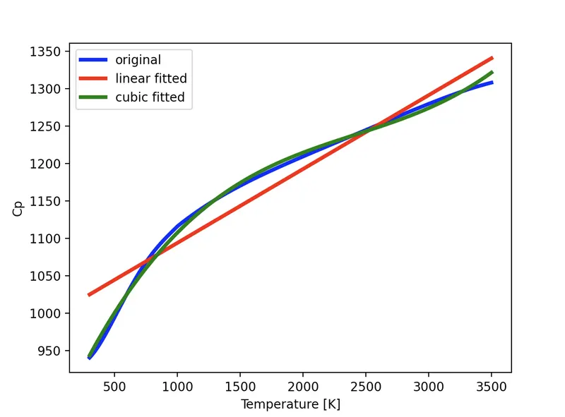
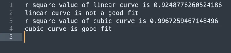
6. r square values were calculated to determine the fit of the functions. from the calculated values it is evident that the cubic function fits the data more accurately than the linear function