Parsing NASA thermodynamic data

Aim:

To write a code in MATLAB that extracts the 14 coefficients and calculates the thermodynamic properties (enthalpy, entropy, molecular weight, and specific heats) of all the species in the data file 'NASA thermodynamic data'.

Theory:

Parsing means breaking it down into component parts so that its syntax can be analyzed, categorized, and understood [1]. By doing this we are going to a string into parts and then recognise the parts to convert it into something simpler than a string. File parsing is to resolve things into component or subpart form and describe the syntactic file. That is, reading in the data stream and building a memory model of it.

NASA Thermodynamic File
NASA came up with polynomials that can be used to evaluate thermodynamic properties such as Enthalpy, Entropy, and Specific heat. They have also documented the coefficients required to evaluate these polynomials for 1000+ species.

NASA thermodynamic file which is the 'THERMO.dat' file contains the temperature range (global), 14 coefficients (both low and high-temperature coefficients) and the local temperature range of the 53 species.

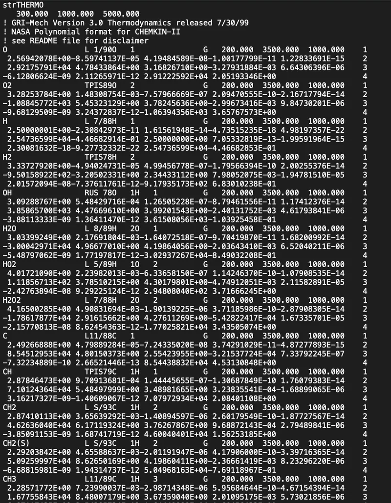
Figure 1: Sample view of THERMO.dat

Figure 1 shows the sample view of THERMO.dat, in this dat file first line is the heading 'THERMO'. The next line is the global temperature range, where 300.000 is the minimum global temperature while 1000.000 and 5000.000 are medium and maximum global temperatures respectively. The next three lines are general information which is not required for the calculation of thermodynamic properties. The next four lines provide the data of the species which is required for the calculation of thermodynamic properties. Out of these four lines, the first line indicates the species and its local temperature range. The next three lines provide the temperature coefficient which is required for the calculation of H, S and Cp. The next four lines are for other species and it is repeated for 53 elements.

The 53 elements in the 'THERMO.dat' file are O, O2, H, H2, OH, H2O, HO2, H2O2, C, CH, CH2, CH2(S), CH3, CH4, CO, CO2, HCO, CH2O, CH2OH, CH3O, CH3OH, C2H, C2H2, C2H3, C2H4, C2H5, C2H6, CH2CO, HCCO, HCCOH, H2CN, HCN, HNO, N, NNH, N2O, NH, NH2, NH3, NO, NO2, HCNO, HOCN, HNCO, NCO, CN, HCNN, N2, AR, C3H8, C3H7, CH3CHO, and CH2CHO.

Thermodynamic Properties
Enthalpy, entropy and specific heat of various species at different temperatures are required extensively to analyze the thermodynamic process. For example, if the combustion process is considered, these quantities are required to observe how the combustion is going on and how efficient or effective is. It then allows seeking to improve the process. Similarly, in other processes like refrigeration, air conditioning, nozzle flow, chemical kinetics, etc, these quantities are widely involved to observe the phenomenon.

Enthalpy
Enthalpy is a property of a thermodynamic system which is equal to the system's internal energy plus the product of its pressure and volume. In a system contained so as to prevent the mass transfer, for processes at constant pressure, the heat absorbed or released equals the change in enthalpy.

Entropy
Entropy is the measure of a system's thermal energy per unit temperature that is unavailable for doing useful work. Because work is obtained from ordered molecular motion, the amount of entropy is also a measure of the molecular disorder or randomness of a system.

Specific Heat
Specific heat is the amount of heat per unit mass required to raise the temperature by one degree Celsius.

Molecular Weight
The average mass of a compound compared to 1/12 the mass of carbon 12 and calculated as the sum of the atomic weights of the constituent atoms.

Atomic Mass
Atomic mass is the mass of a single atom of a chemical element. It includes the masses of the 3 subatomic particles that make up an atom: protons, neutrons and electrons. Atomic mass can be expressed in grams.

The empirical equation to find the thermodynamic properties using the coefficients from the THERMO.dat is provided below:

Enthalpy, `H = RT(a_1 + a_2T/2 + a_3T^2/3 +a_4T^3/4 + a_5T^4/5 + a_6/T)`

Entropy, `S = R(a_1 ln(T) + a_2T + a_3T^2/2 +a_4T^3/3 + a_5T^4/4 + a_7)`

Specific Heat, `C_p = R(a_1 + a_2T +a_3T^2 + a_4T^3+ a_5T^4)`

where, Cp is Specific Heat [J/(K kg)], R is Universal Gas Constant (R=8.314 [J/(mol K)]), H is the Enthalpy [J], S is the Entropy [J/K] and T is the temperature [K].

Objectives:

1. Understanding the theoretical concept of File Parsing and the commands required for it.
2. Writing the program for file parsing.
3. Understanding the concepts of thermodynamic properties and the equations required to calculate them.
4. Incorporating the MatLab code to calculate Entropy, Enthalpy, Specific Heat and Molecular Weight to the main program and plotting the graphs.
5. Save the plots as images with appropriate names and dump them in separate folders for each species with a suitable name.

Program:

The programming is done in MATLAB.

Main code:

%reading header data
clear all 
close all
clc
f1= fopen('THERMO.dat','r');
fgetl(f1);
temp= fgetl(f1)
A= strsplit(temp,' ')

%reading the golbal temp
low_temp= str2num(A{2});
mid_temp= str2num(A{3});
high_temp= str2num(A{4});
fgetl(f1);
fgetl(f1);
fgetl(f1);


c= [];

%reading coefficients of species
while(f1>0)%loop for reading the entire dat file
   temp= fgetl(f1);
   temp= strsplit(temp,' ');
   if sum(strcmp(temp,'END'))%statement to check if file has reached the end point
       break;
   end

   %reading the species name and the local temp
   species_name= temp{1};
   local_low_temp= str2num(temp{end-3});
   local_high_temp= str2num(temp{end-2});
   local_mid_temp= str2num(temp{end-1});
       for i=1:2 %loop for getting the first 10 coefficients
       coefficients= fgetl(f1);
       a= findstr(coefficients,'E');
       c= [c, str2num(coefficients(1:a(1)+3))];
       c= [c, str2num(coefficients(a(1)+4:a(2)+3))];
       c= [c, str2num(coefficients(a(2)+4:a(3)+3))];
       c= [c, str2num(coefficients(a(3)+4:a(4)+3))];
       c= [c, str2num(coefficients(a(4)+4:a(5)+3))];
       end

       %code for getting the remaining 4 coefficients
       coefficients= fgetl(f1);
       a= findstr(coefficients,'E');
       c= [c, str2num(coefficients(1:a(1)+3))];
       c= [c, str2num(coefficients(a(1)+4:a(2)+3))];
       c= [c, str2num(coefficients(a(2)+4:a(3)+3))];
       c= [c, str2num(coefficients(a(3)+4:a(4)+3))];
      
       %creating an array for local low temp range and local high temp
       %range
   low_temp= linspace(local_low_temp,local_mid_temp,100);
   high_temp= linspace(local_mid_temp,local_high_temp,100);


   %calculation of enthalpy/entropy/specific heat
   Cp_high = 8.314*(c(1)+c(2)*high_temp+c(3)*high_temp.^2+c(4)*high_temp.^3+c(5)*high_temp.^4);
   H_high = 8.314*(c(1)*high_temp+c(2)/2*high_temp.^2+c(3)/3*high_temp.^3+c(4)/4*high_temp.^4+c(5)/5*high_temp.^5+c(6));
   S_high = 8.314*(c(1)*log(high_temp)+c(2)*high_temp+c(3)/2*high_temp.^2+c(4)/3*high_temp.^3+c(5)/4*high_temp.^4+c(7));
  

   Cp_low = 8.314*(c(8)+c(9)*low_temp+c(10)*low_temp.^2+c(11)*low_temp.^3+c(12)*low_temp.^4);
   H_low = 8.314*(c(8)*low_temp+c(9)/2*low_temp.^2+c(10)/3*low_temp.^3+c(11)/4*low_temp.^4+c(12)/5*low_temp.^5+c(13));
   S_low = 8.314*(c(8)*log(low_temp)+c(9)*low_temp+c(10)/2*low_temp.^2+c(11)/3*low_temp.^3+c(12)/4*low_temp.^4+c(14));
c=[];

   %creating sub plot for various graphs 
figure(1)
%specific heat plot
subplot(1,3,1)
plot(low_temp,Cp_low);
hold on
plot(high_temp,Cp_high);
title ('Cp data');
xlabel('temp');
ylabel('Cp');
hold off

%enthaply plot
subplot(1,3,2)
plot(low_temp,H_low);
hold on
plot(high_temp,H_high);
title ('enthalpy data');
xlabel('temp');
ylabel('Enthaply');
hold off

%entropy plot
subplot(1,3,3)
plot(low_temp,S_low);
hold on
plot(high_temp,S_high);
title ('Entropy data');
xlabel('temp');
ylabel('Entropy');
hold off


%creation of parent folder and species folder for graphs
z = 'species folder';
mkdir(z);
cd (z);
mkdir (species_name);
cd (species_name); 
saveas(1,'thermo_data.jpg');
cd ..
cd ..
mol_wt= mw_2(species_name);
output= ['molecular weight of ', species_name];
disp(output);
disp(mol_wt);

end

fclose(f1);

Function to calculate Molecular Weight:

function mol_weight= mw_2(species_name)

%all the available molecules
molecules= ['H', 'C', 'O', 'A', 'N'];
m_mass= [1, 12, 16, 40, 14];

weight=0;
%checking each element and adding weight
for i=1:length(species_name)
    for j=1:length(m_mass)
if strcmpi(species_name(i),molecules(j))
    weight= weight+m_mass(j);
    pos=j;
end
    end

%checking for multiple elements
   if (str2num(species_name(i))>1) %error
        num= str2num(species_name(i));
        weight= weight + m_mass(pos)*(num-1);
   end
end
mol_weight= weight;
        

Each step of the program is explained with comments.

The logic of the program

To get access to 'THERMO.dat', the command fopen is used, and to get(extract) the content of each line, the command fgetl is used. The datas from each line is extracted or separated using the command strsplit and each splitted data are actually in character form. In order to change the form on numerical datas from character, str2num [2] command is used. For calculating the thermodynamic properties the datas required such as 14 coefficients, 3 local temperatures (low, medium and high) are extracted. This is calculated using the formula provided for calculating each thermodynamic property. In order to show two regions of low and high temperature range in graph, H_low, S_low and Cp_low (for lower temperature range) and H_high, S_high and Cp_high (for higher temperature range) are calculated. The coefficients are extracted by the logic such that 'E' is found from each line since every coefficient contains E and there are no other Es present. Using mkdir [3], the folder can be created to paste all species and cd is used to change the current folder [4]. With saveas, the graphs are saved in the required folder.

Program Output:

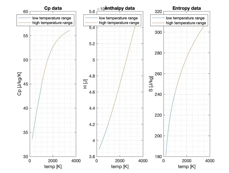
Plots for CH2 species

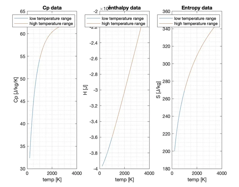
Plots for CO2 species

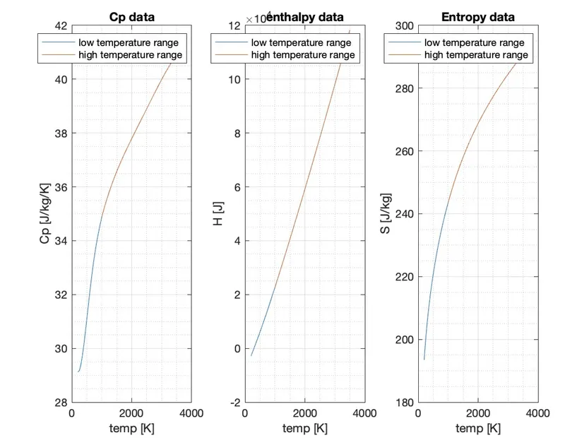
Plots for O2 species

Screenshot of the window where all the folders are saved

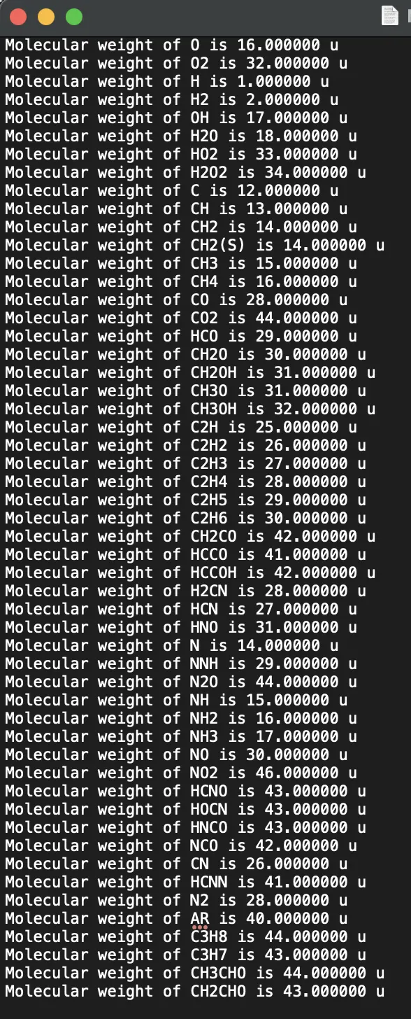
A 'Molecular Weights.txt' file was created using fopen to save the molecular weight of each species calculated using the function 'mw_2.m'. The screenshot of 'Molecular Weights.txt' file is shown below:

Conclusion:

The theoretical concepts of thermodynamics and file parcing has been understood. A program in MATLAB has been created for file parcing. File Parsing is done successfully for the NASA Thermodynamic data and the thermodynamic properties such as enthalpy, entropy and specific heat has also found. The molecular weight of each species has also been found. The thermodynamic properties of each species has been successfully plotted with respect to temperature and is stored in a separate directory using MATLAB code.

References:
[1] https://www.computerhope.com/jargon/p/parse.htm
[2] https://in.mathworks.com/help/matlab/ref/str2num.html
[3] https://in.mathworks.com/help/matlab/ref/mkdir.html
[4] https://in.mathworks.com/help/matlab/ref/cd.html
[5] https://en.wikipedia.org/wiki/List_of_thermodynamic_properties#:~:text=Within%20thermodynamics%2C%20a%20physical%20property,which%20it%20can%20be%20specified.
[6] https://en.wikipedia.org/wiki/List_of_thermodynamic_properties#:~:text=Within%20thermodynamics%2C%20a%20physical%20property,which%20it%20can%20be%20specified.
[7] https://www.thermal-engineering.org/what-is-thermodynamic-property-definition/